
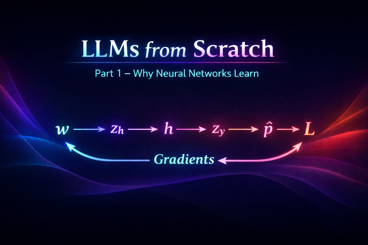
Large Language Models from scratch - Part 1
Or how to deconstruct the discovery of the century in (mostly) understandable parts.

Large Language Models are everywhere now. OpenAI’s ChatGPT took the world by storm in late 2022 and since then the number of LLM’s exploded, whether they be proprietary, open-weights or open-source. At the time of this writing, more than 2.3M models are registered in Hugging Face, 317k alone in the category of ‘Text Generation’. OpenAI reportedly has 800M active weekly users, Anthropic reached 300,000 business customers and approximately 30 million monthly active users for its Claude AI assistant as of Q2 2025. Google’s Gemini App surpassed 650 million users per month, and AI Overviews - the intelligent summary that appears at the top when you do a Google search - now have 2 billion users every month. We’re definitely witnessing a disruptive technology that shows no signs of decelerating.
But what exactly are Large Language Models? How do they work, what are their mathematical foundations, how do they differ from each other, but most importantly: what are the steps to build one from scratch? That's the goal for these series of posts that will be as comprehensible as possible. There are a lot of not so trivial concepts that one needs to be comfortable with in order to grasp the core ideas behind LLM’s, and what better way to understand the process than actually developing one from scratch? The idea is to simplify as much as possible the theory, reducing it to its first principles, but at the same time deliver an organic whole that encompasses state-of-the-art techniques not too far away from production grade LLM’s. Of course, training a production grade model requires substantial investment, so we will adapt for it to be manageable in consumer-grade hardware.
What’s on the menu on this part?
Machine Learning Models
Neural Networks
Neural Network Inference
Neural Network Training
Let’s begin.
What you see today when you interact with ChatGPT is a rather simple system: there’s a chat input where you write what you want the model to answer to, hit enter, and then you wait for the model response. Depending on the model you can also upload documents, images, sound as a context to the chat prompt; you can also select whether you want the model to “think” harder, do a “deep research”, search the web, etc. But in the end of the day you have a system that receives an input, and a black box that ruminates on that input and outputs an answer.
But, what’s in that box?
For the purpose of our reflexion we will consider that behind such a system is only one model. As you will see, a production-grade such system may rely on several models, not just one and not all from the same type, but we will focus our analysis specifically on one type of model: a Large Language Model.
Machine Learning Models
An LLM, as the name implies, is first and foremost a Language Model that is Large. When we say Language Model we mean a Machine Learning Language Model. A Machine Learning model is what you end up with when training an algorithm on data, typically lots of it, being essentially a complex function that learns patterns in the training data to then make predictions or decisions on new, unseen data without explicit programming for every scenario. In this regard we can say that a machine automatically learns and generalizes it’s understanding of the training dataset it was fed with in the first place and is able to answer, most of the time correctly, on data that it has never seen.
Machine learning algorithms are typically divided in 3 types:
Supervised Learning: Learns from labeled data (input-output pairs) to predict outcomes. It’s normally used in two types of problems that mostly differ on whether the results are discrete or continuous: classification problems - where the response belongs to a set of classes (e.g., spam detection) - and regression problems - where the response is continuous (e.g., house price prediction).
Unsupervised Learning: Finds patterns in unlabeled data, often grouping similar items (clustering).
Reinforcement Learning: Learns through trial-and-error, receiving rewards or penalties (e.g., autonomous driving).
Each type has its own set of machine learning algorithms: for classification problems the most popular ones are typically: Support Vector Machines (SVM), Decision Trees, Ensemble Trees, Naive Bayes, k-Nearest Neighbors (KNN), and…Neural Networks.
For regression problems the most popular ones start with Linear Regression, Polynomial Regression, Decision Tree Regression, Random Forest Regression, Support Vector Regression, and… Neural Networks.
As you can see there are lots of machine learning algorithms. I should make an honorary mention of XGBoost, that is normally considered the swiss army knife of the ML algorithms, with an excellent track record for both classification and regression problems. It’s an Ensemble Trees method that normally combines several decision trees - also called weak learners - and then aggregates the result using a boosting technique: trees are built sequentially, with each new tree focusing on correcting the errors of the previous ones. There are at least two more techniques regarding the Ensemble Trees method: bagging, trains multiple trees independently on different random subsets (with replacement) of the training data (Random Forest is a good example of this), and stack/voting, that trains different types of models (or same type with different parameters) and uses a meta-model or voting to combine their final predictions.
Deep diving on each and every one of these algorithms is outside of the scope of our analysis, but we will go in much deeper in just one of them because it’s at the root of LLMs: Neural Networks.
Neural Networks
Artificial Neural Networks (ANN) are fascinating. They’re directly inspired by the biological brain, composed by a network of neurons that communicate via electrochemical signals. Artificial neurons, or nodes, receive input signals, process them, and pass them to other nodes. Biological neurons pass information, or “fire”, when the input signal exceeds a certain threshold, and that’s exactly what happens with artificial neurons: they use activation functions that decide whether they should “fire”. The concept of artificial neurons goes way back to the 40’s with Warren McCulloch and Walter Pitts creating the first mathematical model of an artificial neuron. The field has been advancing since then with the development of the Perceptron, the introduction of the backpropagation algorithm, and a whole series of different and evermore sophisticated ANN architectures.
Let’s start with a simple example. Consider the following ANN:
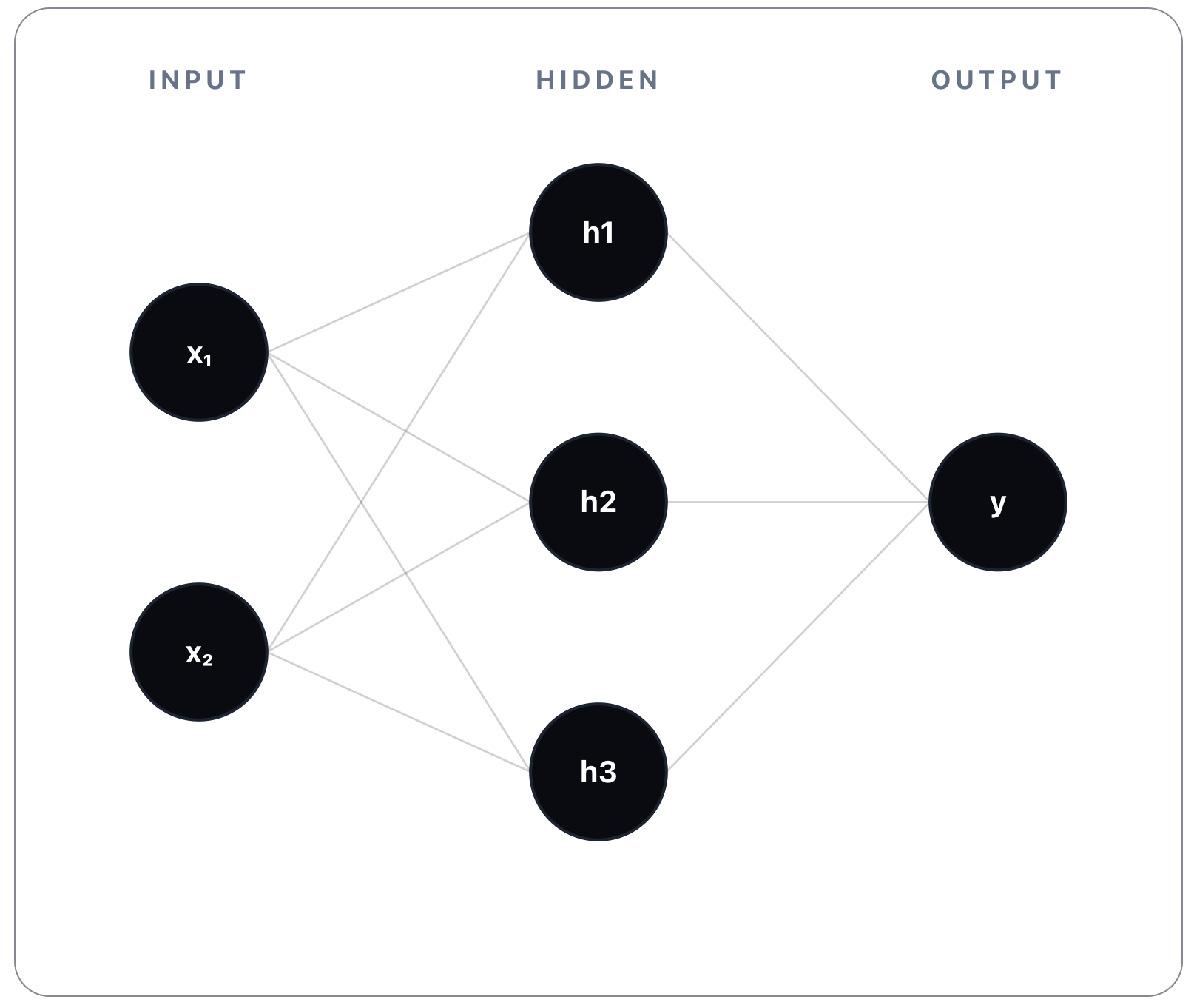
This network has an Input Layer, one Hidden Layer, and an Output Layer. Typically all neural networks have one Input and one Output layers, and one or more Hidden layers. As the name implies, the input layer holds as many neurons as needed for the input data of the problem at hand. Similarly, the output layer will hold as many neurons as needed for holding a prediction result. The hidden layers represent the network’s core feature extraction (more on this in a bit) capability, essentially being where all the computation work is done. The number of nodes on each hidden layer, and the number of hidden layers, is perfectly arbitrary. It really depends on the problem we want to solve, but generally the more hidden layers there are, the deeper the network is (hence the notion of deep learning, applied to deep neural networks), and the more each hidden layer learns increasingly abstract representations of the data that flows from one hidden layer to the next.
The way information flows from the input to the output layer - also called a forward pass - and from one node to another node is by performing linear calculations and a function activation:
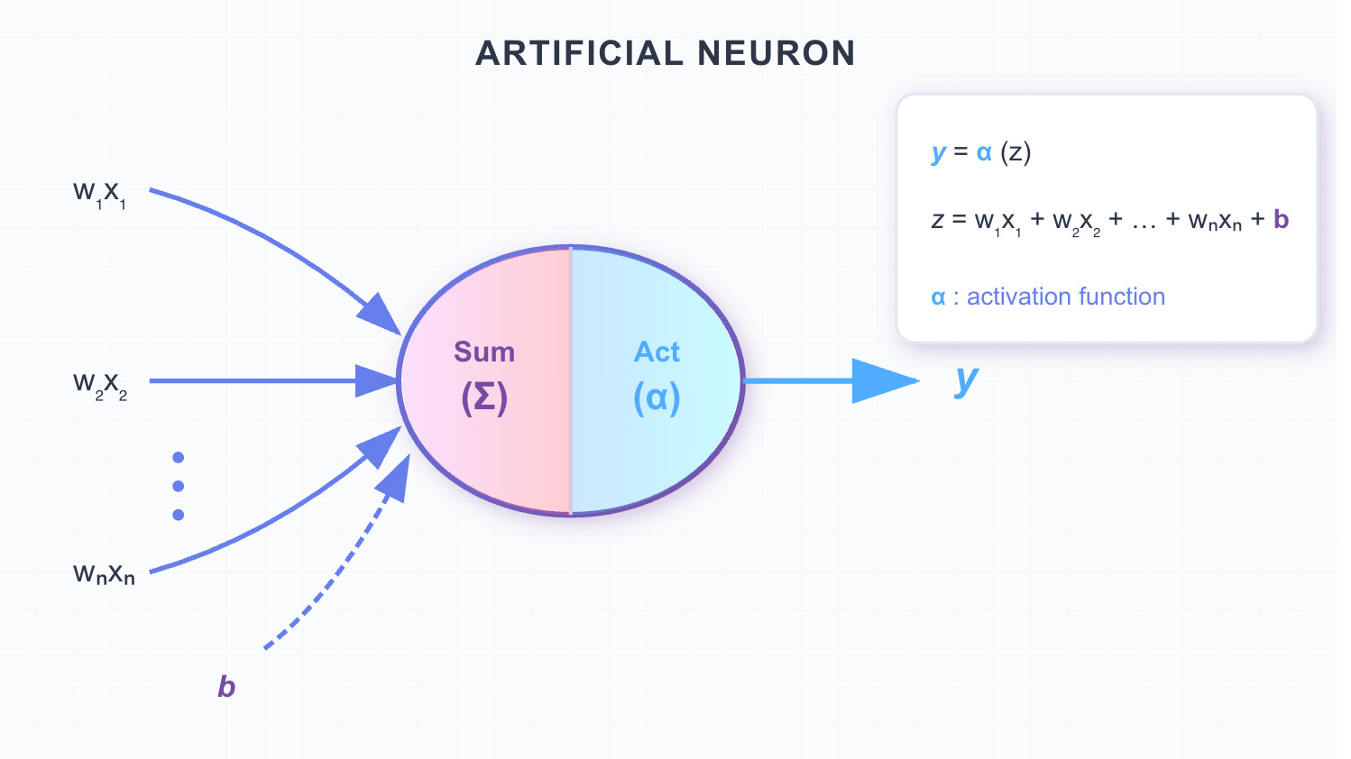
Each neuron performs a linear calculation based on all its input connections and a function activation on the result of the linear calculation.
First it sums up all the information coming in the neuron:
Where:
Input / Feature: The data being fed into the neuron. We will get back to this feature notion a bit later.
Weight: Determines the importance of each input feature. It acts as a slope, controlling how strongly the input influences the output.
Bias: A trainable parameter that shifts the activation function left or right, allowing the model to fit data that does not pass through the origin. It mostly adds flexibility in what would otherwise be just a sequence of multiplications.
Pre-activation / Linear Combination: The result of the linear transformation before applying the activation function.
Lastly we apply the activation function:
Where:
Activation function: sigmoid, ReLU, tanh, softmax, etc. These non-linear functions introduce non-linearity in what would be just a sum of linear equations, collapsing all hidden layers and severely impacting the network’s ability to learn complex patterns in data.
The final result that is passed to the next node.
Neural Network Inference
Let’s apply a simple problem to the example we gave earlier that hopefully will put these simple calculations into some context. Consider the scenario of a student that needs to pass a final exam, having attended its respective classes and having studied for some hours per day. We consider x1 is the number of hours a student studies per day, x2 is the percentage of class attendance, and we want to predict if the student will pass or fail the exam. There are several ways to model even this simple problem, we could try to infer the actual continuous score of the exam from 0-100%. Or to infer the discrete grade - from A to F - or just infer that he will pass or fail the exam, as a binary classification. These three different outcomes imply three different output layers, activation functions and, as we will see, loss functions. But we will stick to the simplest example and predict simply whether the student will pass or fail the exam.
Let’s consider, as an input example:
x1: 5 hours
x2: 60%
So the student studied 5 hours a day and attended 60% of classes. Let’s find out if, according to the network, he will pass or fail the exam.
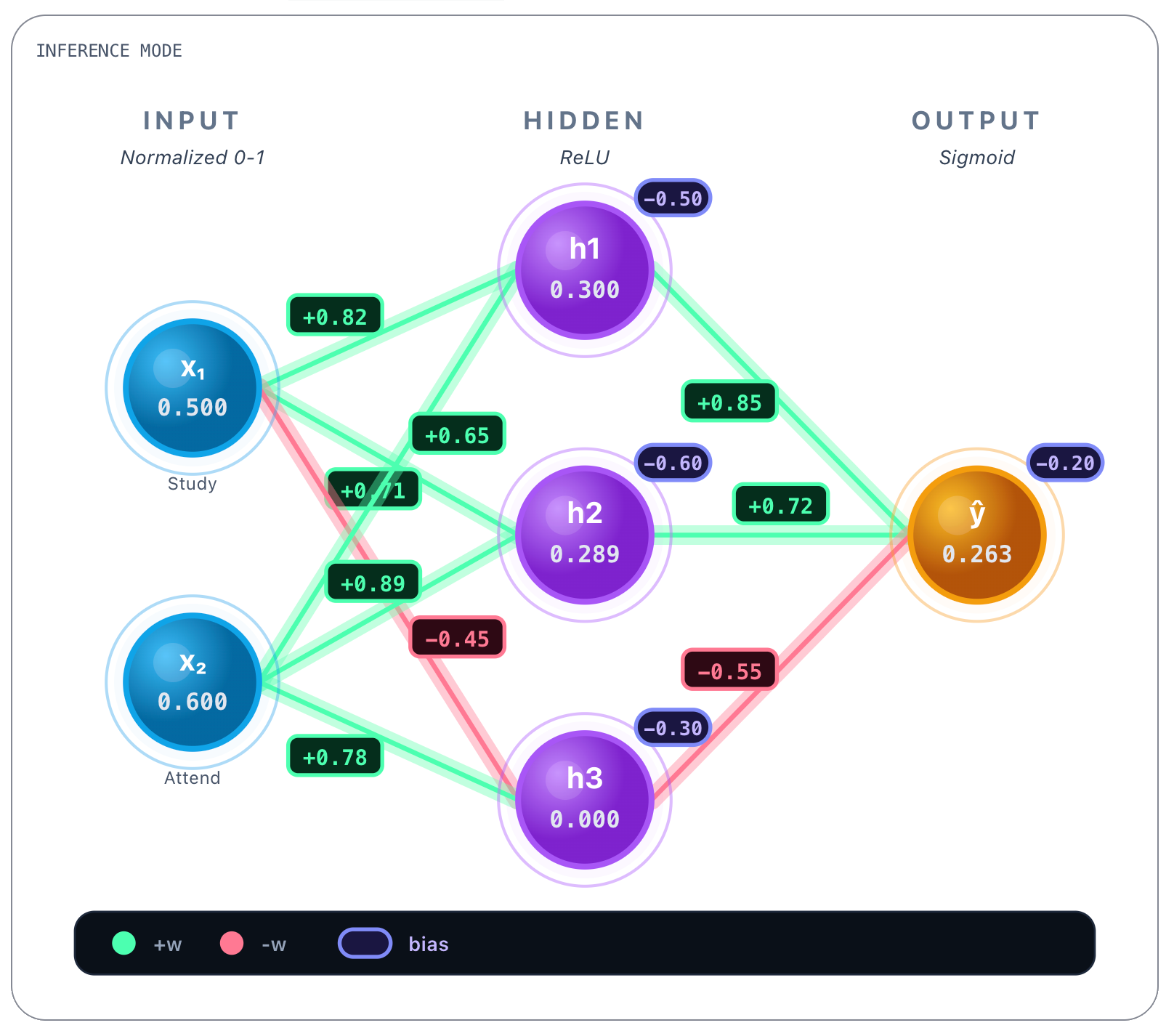
An already trained network behaves like this:
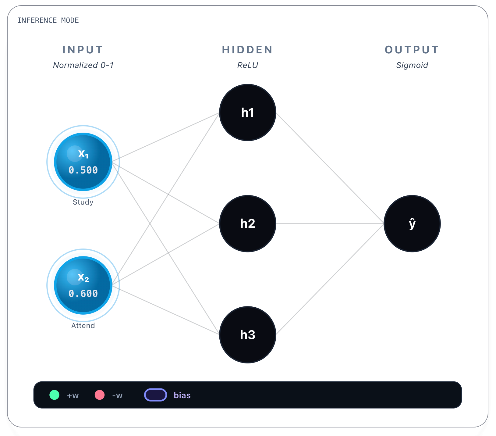
We input both variables in the Input layer. Notice that both x1 and x2 are normalized values between [0, 1]. To normalize the x1 value we consider 10h as a maximum value, so 5h is 50%, or 0.5. Regarding attendance, 60% is already in the [0,1] interval. It’s important that all the values be normalized so both inputs contribute proportionally and no feature dominates the others.
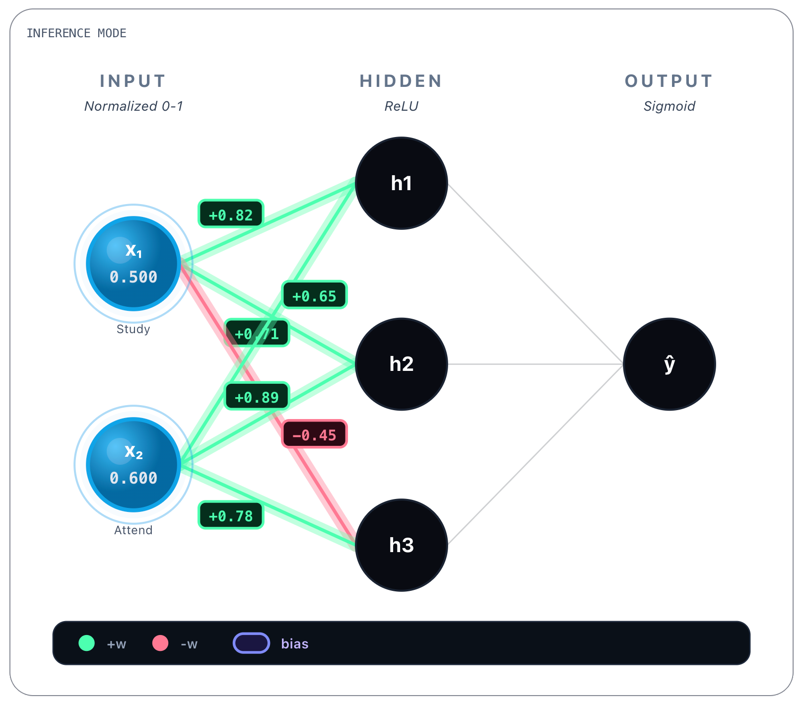
Then for each connection between every input node and a hidden layer’s node there’s a weight value attributed to that connection. In the picture above you can see, for instance, between x1 and h1 the value of +0.82. And between x1 and h3 the value of -0.45. Each connection then has a learned weight:
From Study Hours (x₁):
  → h₁: w = 0.82
  → h₂: w = 0.71
  → h₃: w = -0.45
From Attendance (x₂):
→ h₁: w = 0.65
→ h₂: w = 0.89
→ h₃: w = 0.78These values were obtained during training and are static once the network is trained. Whatever the inputs, these values are always the same. Bias values are also learned and static, we show them next.
Biases: [-0.50, -0.60, -0.30]You can see biases on the top right corner of each hidden layer’s node.
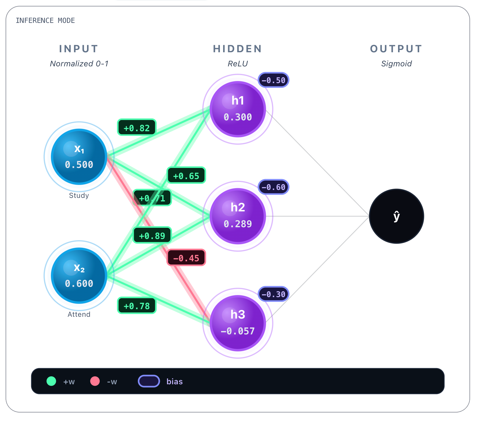
Next we perform linear calculations referenced earlier, so for each hidden layer’s node we compute the following for every incoming connection:
And we obtain the following values, that you can see in the picture on each h1, h2 and h3 nodes:
h₁: z = (0.82 * 0.500) + (0.65 * 0.600) - 0.50 = 0.3000
h₂: z = (0.71 * 0.500) + (0.89 * 0.600) - 0.60 = 0.2890
h₃: z = (-0.45 * 0.500) + (0.78 * 0.600) - 0.30 = -0.057
So now, after linear calculations you can see each result on each hidden layer’s node. Now we perform the ReLU function activation over each hidden layer node result as we stated earlier:
Which in ReLU’s case:
ReLU is an acronym for Rectified Linear Unit. Basically resets negative values to zero and lets through positive values. We could’ve chosen other functions, there are various alternatives, we will go deeper on this later.
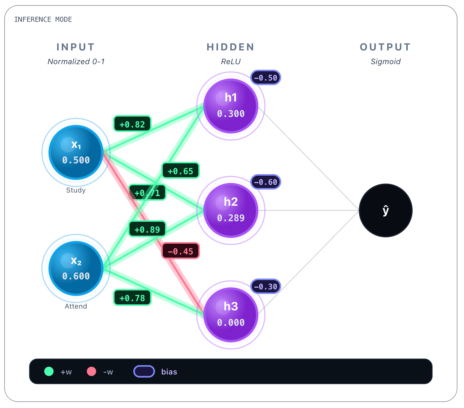
As you can see, looking to h1, h2 and h3 nodes, only node h3 changed value from a negative value -0.057 to 0. This is because, as we said earlier, ReLU resets negative values to zero and lets through positive values. That was what happened to h1 and h2 nodes, whose value stayed the same. So at this point on each h1, h2 and h3 we have final linear calculations plus ReLU activation function results.
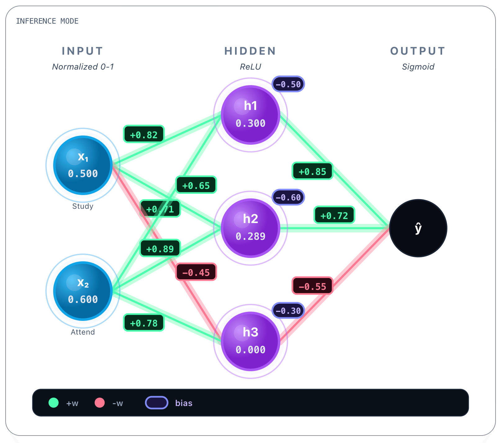
Next we continue, doing the same calculations per connection. The next connection’s weights obtained in training:
h₁ → output: w = 0.85
h₂ → output: w = 0.72
h₃ → output: w = -0.55
Bias we reveal next.
Output bias: b = -0.20Now we perform the same computation again, this time from h1, h2 and h3 values computed earlier as our Input / Feature values:
z = (0.85 * 0.300) + (0.72 * 0.289) + (-0.55 * 0) - 0.20 = 0.2631Now we apply another activation function, this time we choose to apply the sigmoid function, that squashes values to probabilities between [0,1]:
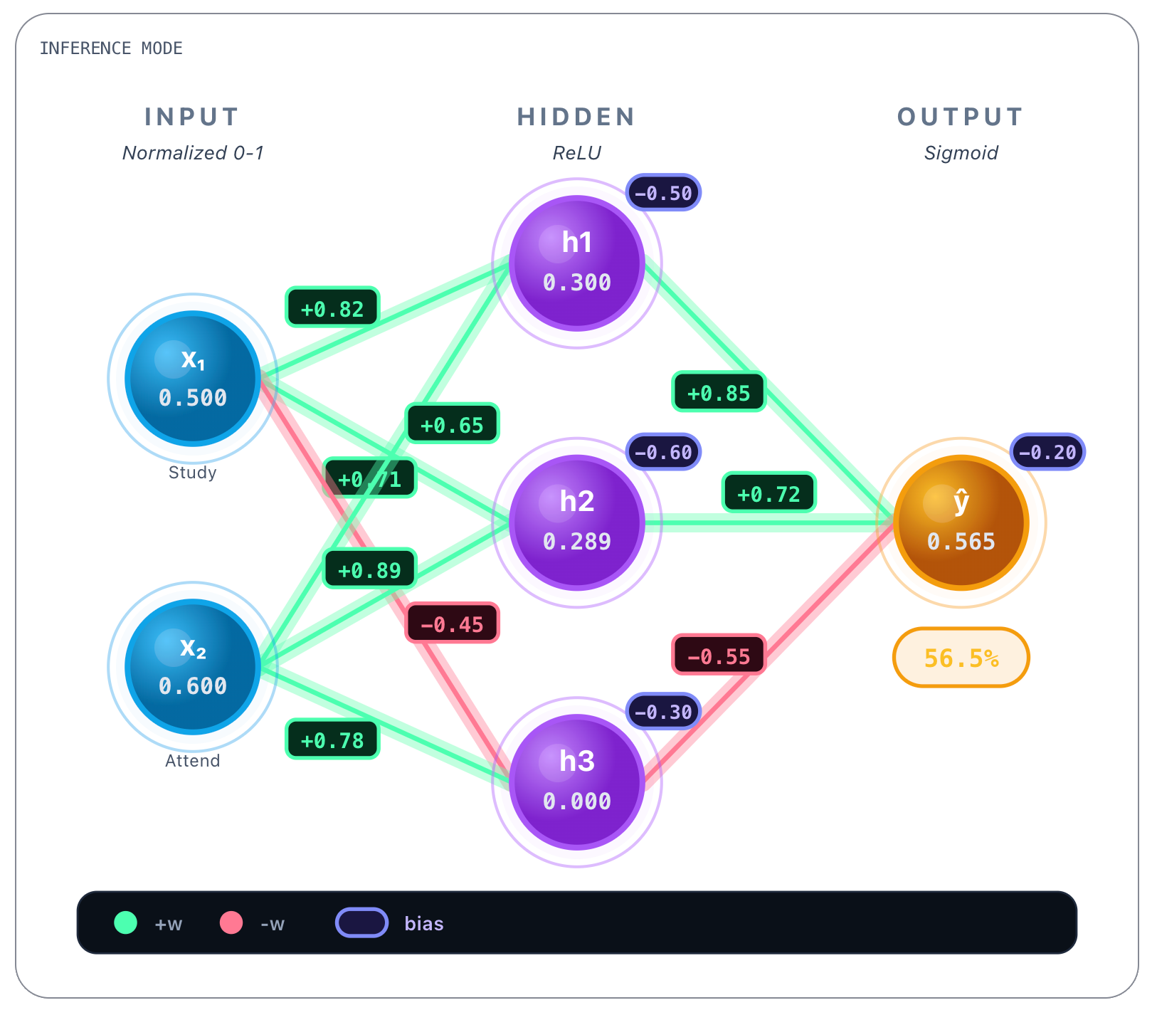
Applying the sigmoid function to the obtained value 0.263:
We end up with the full prediction of the network for the first question, that was to know if the student passed or not given that the student studied 5 hours per day and attended 60% of classes: 56.5%. So yes, the student would pass (barely).
You can see that choosing sigmoid as activating function in the output layer was not innocent. Even though the prediction only required some way of performing binary classification - pass / fail - the network’s output values are always continous - we will see why in a bit - and therefore we settle anything equal or above 0.5 as passing the exam, anything lower than that, means the student fails the exam.
As you can see, aside from some probably unfamiliar functions, the core network’s calculations are really simple to follow along. But what you are seeing is just an already trained network doing inference. But how was the network’s trained ?
Neural Network Training
This will be a bit trickier, but we will go through step by step as we did in inference. It’s very, very important that we nail these building blocks with very basic networks because from here things will get a lot more complex so we need to be very clear on the fundamentals.
Let’s dive in.
For training a neural network, or any other kind of model, we generally need three datasets: training, validation and test datasets. Usually they’re segmented over the total collection of observations of the reality we want to model, for instance: 80% training, 10% validation, 10% test. For big data 90% training, 5% validation, 5% test is also common. For all datasets we must sample from the same distribution:
To put it in another way: validation and test are “small versions of reality”.
training is “what the model studies”. So one must strive to keep the same diversity found globally in the studied reality on each and every one of the datasets, otherwise we’re modeling different “realities” making the process unfruitful. This process is also called stratified sampling, A stratified sample is a way of splitting data so that each subset keeps the same structure as the full dataset. Instead of sampling randomly, we preserve the proportions of important groups (called strata).
The validation process is stateless, during validation the model is freezed and there are no weight updates, only in the training process weights get updated. In this regard, and generally speaking, the validation dataset is normally used to tune the training algorithm’s hyperparameters/early stopping - because you train the model over the training dataset with a specific hyperparameter config and then you validate this model/configuration agaisnt the validation dataset. It’s from this match that is calculated the validation loss, i.e., the average error the model makes on the validation dataset and is used to estimate how well the model generalizes, because this dataset was not seen in training data. The training loss is the same error, but is calculated over the training dataset and it is the quantity that is minimized during learning.
The training loss:
The validation loss:
Where:
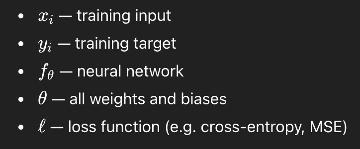
These are rather simple equations: we just apply the loss function to the real observed value - the training target - and the prediction of the network - that is, the complex function that receives an input x and gives an output f(x) by performing the linear calculations you saw earlier in the inference example - (we will see some loss functions in detail, particularly cross-entropy and mean squared error (MSE)). We sum all those loss values and divide by the number of elements in the dataset to get the average value.
We will keep training, trying to reduce both the training and the validation losses, that is, trying to minimize the errors the model obtains while trying to model the reality we’re interested in. Training loss normally goes down as the training progresses, but validation loss can down or go up. If that happens, it’s a clear signal of overfitting, that is, the model keeps reducing the loss over the training set, but is no longer generalizing well to unseen data. It’s being overfitted to the training set, modeling noise instead of signal. When this happens, the training process may stop early.
Once the model is trained and validated, it can finally be evaluated on the test dataset, a subset the model has never seen during the entire process, and conventional metrics are calculated: accuracy, precision, recall, F1-score, etc. The model training process ends here.
All of these concepts could also be applied to other machine learning algorithms, they’re not exclusive of neural networks, but are necessary to have a full picture of the scope of work. Let’s now see effectively how a neural network is actually trained. We will just focus on the core training mechanics, essentially seeing how weights get updated when processing a training dataset.
To go back to the same student problem we tackled before, consider this training dataset:
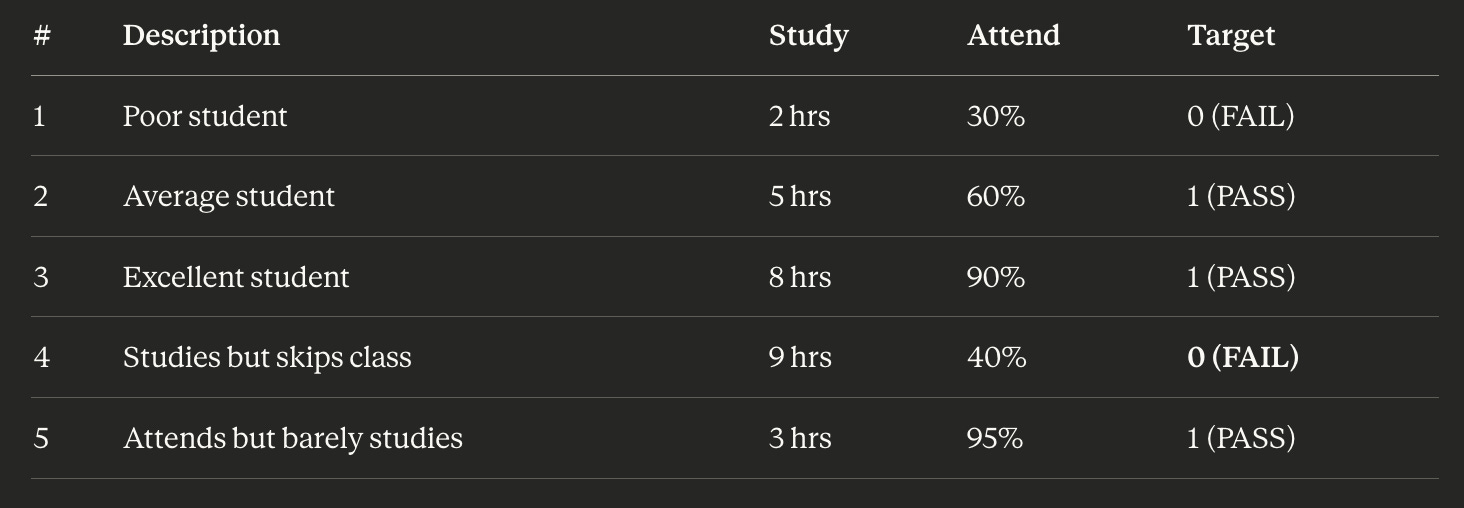
Here we see quite a few observations of the reality we are trying to model. We see a student that doesn’t study very much nor attends class (and inevitably fails the exam). We see an average student, an excellent student, and examples of both extremities: a student that studies but skips class, and vice-versa, one that attends but barely studies. If you notice, all of the cases have targeted observations: all have pass/fail outcomes. It’s as if this is an historical record of student behaviours and their respective exam outcomes. This is our observable reality, it’s by mining this list and showing to a network a comprehensive set of examples that try to describe in it’s more complete form the observable reality we want to model, that we effectively teach the network to discern the relation between hours of study, class attendance, and final exam outcome. And the network, with enough examples and training, will learn it automatically.
As we said earlier, for effectively training a model we also need a validation and test datasets, but for now we will only concentrate in the core training algorithm and on how the training process uses the training dataset.
So the training process will iterate on every example of the training dataset multiple times. We say that when a model has trained over the entire dataset - that is, that saw all the examples contained in the dataset once- that it completed 1 epoch. Training often involves multiple epochs because error minimization and weight updating is an iterative process. It’s as if the network was studying a book and it read the whole book several times, not just one. More epochs means more learning, until it starts memorizing, which is not good, because the network stops learning the underlying patterns and starts learning data itself which leads to overfitting and thus poor generalization.
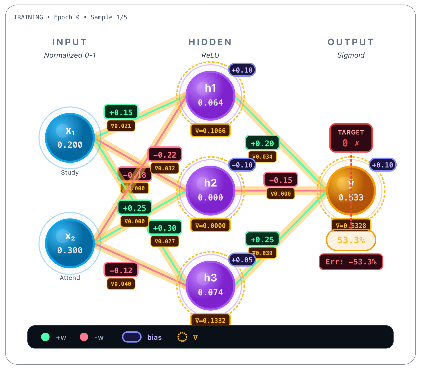
Let’s start by picking the first example of the dataset, the poor student, that studied 2 hours/day and only attended 30% of classes, having failed the exam. Normalized values are, respectively, x1 = 0.2 and x2 = 0.3 :
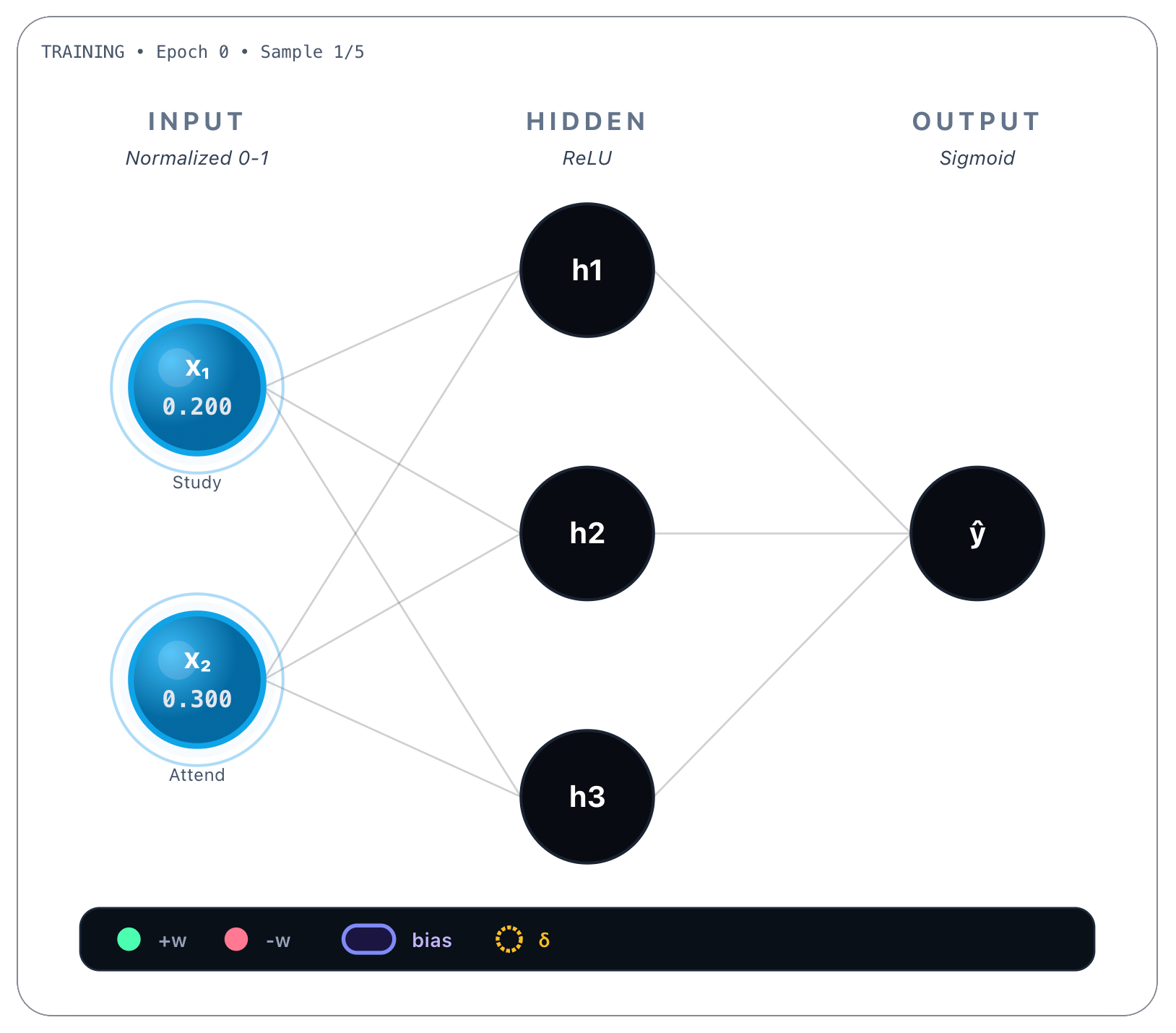
Now we do a forward pass, that is, we perform all the previous calculations we saw earlier as if we were inferencing, this time with random weights.
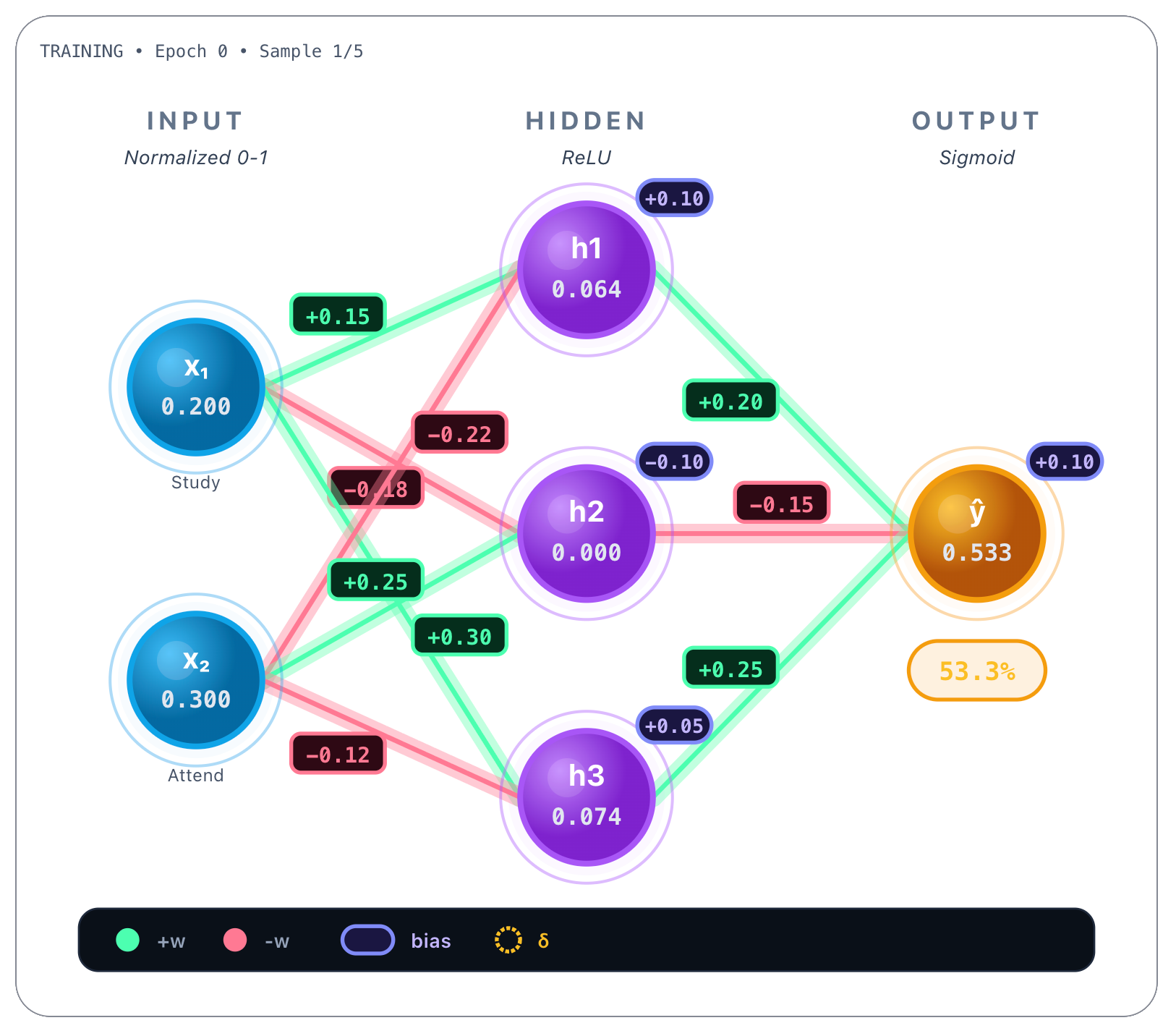
Here the model predicted that a poor student would pass the final exam, because the network’s output was 0.533, that is >= 0.5. But remember that the target score was 0, not 0.533, so the student, as observed, failed the final exam:
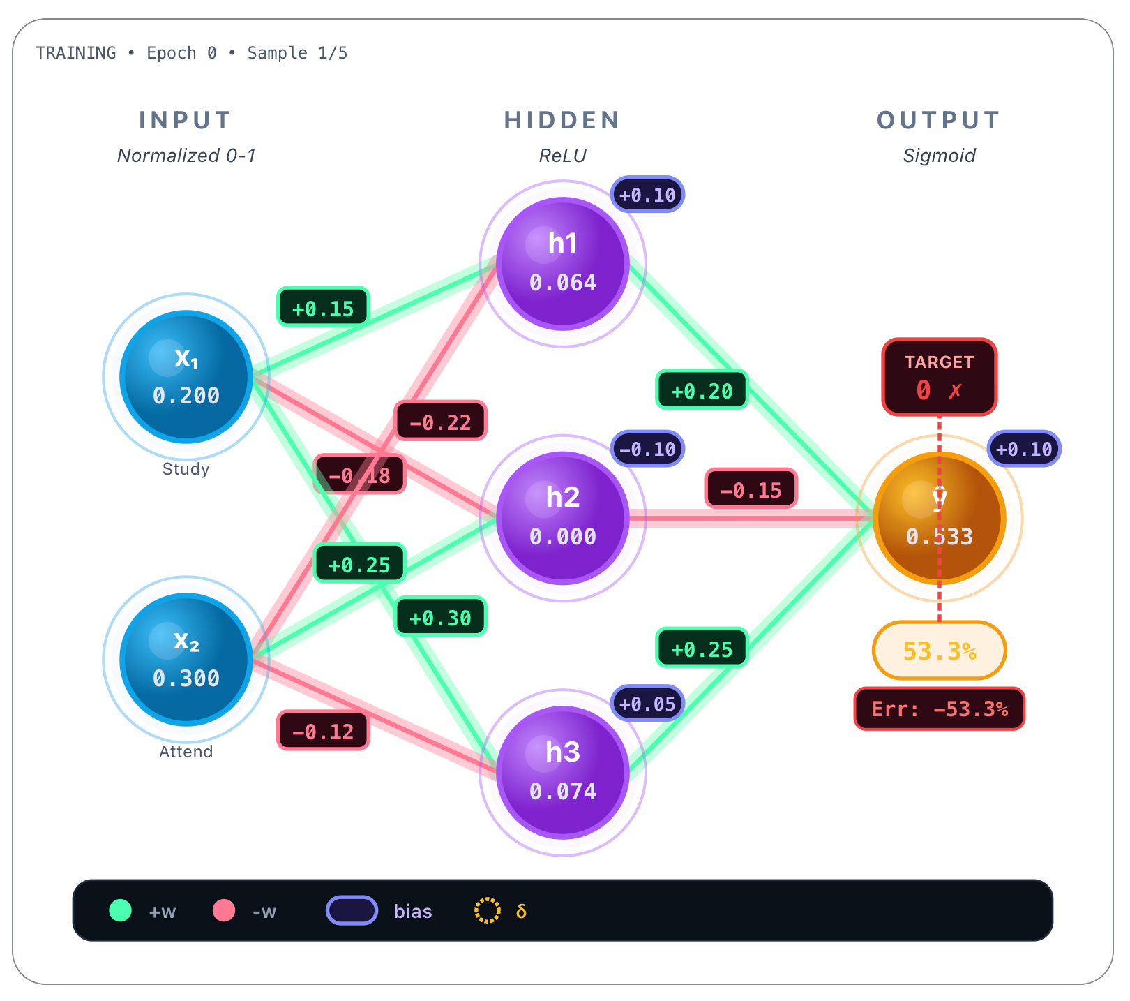
So we have an error of -53.3%, the difference between the predicted value: 53.3%, and the target value the network should’ve predicted: 0 (fail). Now the idea is to update all the weights of the network in such a way that we minimize this error. In order to do that we will compute the training loss as we saw earlier and use a cross-entropy function, in this case, binary cross-entropy:
Binary cross-entropy loss is tipically used in binary classification problems, but why use this function and not something else, and what is this thing really? Let’s take a look.
When we train a neural network for a binary classification problem, we are trying to answer a question that sounds extremely simple: yes or no. Did the student pass the exam or not? Is this email spam or not? Is this transaction fraudulent or legitimate?
Even though the final answer is binary, a neural network never works with hard “yes” or “no” decisions internally. Instead, it always produces continuous values (more on this in a bit). In the case of binary classification, the network usually outputs a number between 0 and 1. This number is best understood as a degree of belief. When the model outputs 0.9, it is saying “I believe there is a 90% chance this is a yes.” When it outputs 0.1, it is saying “I believe there is a 10% chance this is a yes.”
This is why the sigmoid function is so commonly used at the output layer: it guarantees that the network’s output stays between 0 and 1, which makes it naturally interpretable as a probability. However, there is an important distinction here. While the model outputs probabilities, the training data does not. The real world does not give us probabilities; it gives us outcomes. A student either passed or failed. An email is either spam or it isn’t. So the training labels are always discrete values: 0 or 1.
This type of situation is perfectly described by something called a Bernoulli experiment. A Bernoulli experiment is the simplest kind of random experiment imaginable. It has only two possible outcomes: success or failure, yes or no, 1 or 0. A Bernoulli distribution simply says that there is some probability p that the outcome is 1, and a probability 1 - p that the outcome is 0. That’s all it is. In binary classification, the world generates Bernoulli outcomes, and the neural network’s job is to estimate the probability p.
At this point, we need a way to measure how good the model’s predictions are. This is where the concept of likelihood comes in. Likelihood answers a very intuitive question: given what the model predicted, how plausible was what actually happened? If a model predicts a 95% chance of passing and the student passes, that outcome feels very reasonable. If the model predicts a 2% chance of passing and the student passes, that outcome feels surprising. Likelihood is simply a way of quantifying that feeling of surprise.
During training, we want the model to make the observed outcomes as plausible as possible. In other words, we want to maximize the likelihood of the data under the model’s predictions. However, there is a practical issue: probabilities multiply when we look at many data points, and multiplying many small numbers quickly becomes numerically unstable. To solve this, we take the logarithm of the likelihood. Logarithms turn multiplications into additions, making the math more stable and easier to optimize. There is another benefit: probabilities close to zero turn into very large negative numbers when we take the log, which means confident mistakes are heavily penalized.
Because most optimization algorithms are designed to minimize a quantity rather than maximize it, we simply negate the log-likelihood. This gives us what is called the negative log-likelihood. In plain language, negative log-likelihood measures how surprised the model is by reality. The more surprised it is, the larger the loss.
Now comes the key connection. When the outcomes follow a Bernoulli distribution — meaning the labels are 0 or 1 — the negative log-likelihood simplifies into a very specific mathematical expression. That expression is what we call binary cross-entropy. For a single data point, it looks like what we already showed :
This formula has a very intuitive interpretation. Let’s dissect it a bit where each symbol means:
y is the true label (either 0 or 1)
y=1 means “YES / positive class”
y=0 means “NO / negative class”
p(hat) is the model’s predicted probability that the label is 1
e.g. p(hat)=0.90 means “90% chance it’s class 1”
Now let’s see how this formula behaves in the two possible cases.
If the true label is 1, that is, y = 1, the loss depends only on:
A high value of p(hat) means the log is close to 0, so -log is tiny which is good. But if p(hat) is low, the log is actually a very large negative number so -log is huge. You are punished if the model assigned a low probability to something that actually happened.
If the true label is 0, that is, y = 0, the loss depends on:
Here the reverse thing happens. If p(hat) is low, the result will be tiny. If it’s high, the result will be huge because log will approach zero. You are punished if the model was confident in the wrong direction. Confident and correct predictions lead to very small losses, while confident and wrong predictions lead to very large losses. This is exactly the behavior we want when training a classifier.
A word about the word entropy in “cross-entropy”. It comes from information theory, where entropy measures uncertainty or unpredictability. Low entropy means outcomes are easy to predict; high entropy means they are unpredictable. The word cross is there because we are comparing two different probability distributions: the true distribution that generated the data, and the distribution predicted by the model. Cross-entropy measures how inefficient it is to describe reality using the model’s probabilities instead of the true ones. Training a model by minimizing cross-entropy is equivalent to making the model’s predicted distribution match reality as closely as possible.
This is why binary cross-entropy is the standard loss function for binary classification. It matches the nature of the data, it trains the model to produce meaningful probabilities, it strongly penalizes confident mistakes, and it works perfectly with sigmoid outputs. In simple terms, binary cross-entropy teaches a model to be honest about uncertainty when the world only gives yes-or-no answers.
Now, remember when we said the output of the network are always continuous ? Well there’s another particularity that loss functions must follow: they must all be differentiable. But why?
Let’s first see what “differentiable” means: a function is differentiable if you can compute its derivative (slope) everywhere. Formally, this needs to exist:
That means:
The function is smooth
No sharp corners
No jumps
No flat pieces with no slope
A brief note on derivative. A derivative measures how fast a function changes at a particular point. Intuitively, it tells us how sensitive the output of a function is to small changes in its input. Geometrically, the derivative at a point corresponds to the slope of the tangent line to the curve at that point. The tangent line is the straight line that just touches the curve at a single point and best approximates the function near that point. While the curve may bend and change direction, the tangent line captures its instantaneous direction and steepness exactly at that location.
In the context of neural networks, the loss function depends on many parameters, and derivatives tell us how sensitive the loss is to each weight or bias. By computing these derivatives, we understand how small adjustments to parameters affect the model’s error, which is precisely the information needed to guide learning. In this sense, derivatives provide the local compass that allows optimization algorithms to navigate the complex landscape of neural network training.
Back to “differentiable” concept.
The loss function needs to be differentiable because training employs the most common learning algorithm: gradient descent. It works by computing the derivative of the loss with respect to (wrt) each model parameter (or model weight, it’s the same) and then nudging those parameters in the direction that reduces the loss. If the loss function were not differentiable, there would be no reliable way to know whether a small change to a weight improves or worsens the model. Learning would simply not be possible.
Formally, gradient descent is defined as follows:
Where:
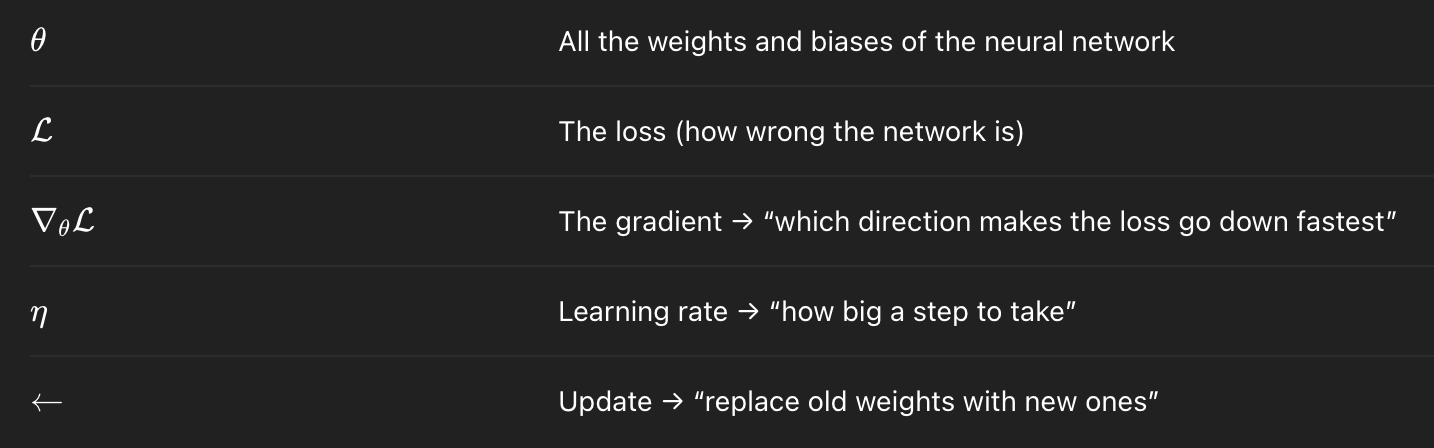
Great. But what is the “gradient” ? The gradient is a vector of partial derivatives that tells you how much the loss changes when each weight changes. Formally:
Each partial derivative tells you: “If I move a tiny bit in this coordinate direction, does the function go up or down?”
When you combine them into a vector, you get the direction that increases the function the fastest.
But in the gradient descent equation notice the minus sign. The gradient points uphill, that is, the direction of the steepest increase:
But we want to go downhill (reduce the loss).
So we move in the opposite direction:
To give you a clearer mental image, imagine you’re on a foggy mountain and want to reach the valley.
You can’t see the whole landscape
You only feel the slope under your feet
So you:
Feel which way goes downhill (gradient)
Take a small step that way (learning rate, n)
Repeat
Eventually you reach the bottom. And this works because the loss function is:
Smooth
Differentiable
Shaped like a bowl
We call the process of calculating the gradient backpropagation, and we call gradient descent the rule by which we actually update the weights using the gradient vector.
A neural network is a function with thousands or millions of parameters. The loss is therefore a function of many variables. Training the network means computing how sensitive the loss is to each parameter, that is, finding out the partial derivatives of the loss function with respect to each weight, and form the gradient vector, which tells us how to move in parameter space to reduce the loss.
The way backpropagation helps achieve this is by applying a rule called the chain rule, that intuitively works like this: if something depends on something else, which depends on something else, then the rate of change is the product of all intermediate changes. Or in other words, the chain rule says that when a quantity depends on another through a sequence of transformations, its derivative is the product of the derivatives of each transformation. Neural networks are nothing more than long chains of functions, so backpropagation is simply the chain rule applied repeatedly.
But how do you effectively calculate the gradient vector ? Let’s continue.
As we were saying, the target is 0 and the predicted value is 0.533. So we substitute those two numbers, y and p(hat) in the binary cross-entropy equation when the true label is 0 :
This is the loss value. For sigmoid output with BCE, the derivative wrt the logit (that is, the raw score before sigmoid activation) is:
So:
This number is the “error signal” at the output.
So what we will do now is to calculate, according to the chain rule, the derivatives of all the forward dependency chain, starting on the weights connecting the hidden nodes, the hidden nodes and their activations, the output weights, the prediction, and effectively the loss function:
Formally:
So let’s begin by calculating the gradients for the weights that connect the hidden layer’s nodes h1, h2 and h3, and the output.
For each output weight the derivative is like this:
And for the output bias, the derivative is:
So the calculated gradients for all the hidden → output nodes:
We now calculate the gradients for hidden nodes. Don’t forget that hidden nodes have a ReLU activation function. First derivative also includes it, and is like this:
The ReLU derivative being:
The ReLU derivative for each hidden layer neuron is like this:
Gradient values for hidden nodes:
We now finally calculate the gradients for all the weights that connect the input nodes and the hidden layer’s nodes.
The first derivative is for the input weights is like this:
And for the hidden nodes bias:
So the gradients for the weights connecting to the hidden neuron h1 are calculated like this:
And the gradients for the weights connecting to the hidden neuron h2 are calculated like this:
Finally, the gradients for the weights connecting to the hidden neuron h3 are calculated like this:
Having calculated all the gradients, we now perform the gradient descent update on all weights.
Recalling the formula, the gradient descent update rule is:
So each weight updates like this:
Considering the learning rate as 0.5, here are the hidden nodes → output weight updates:
Now, for the hidden node h1 updates:
The hidden h2 suffers no updates:
And finally the hidden h3 node updates:
All of these calculations are in fact what the gradient vector is all about: all the individual gradients stacked together. Formally:
And with filled in values:
So the gradient descent in vector form is like this:
Whew, and finally after all these calculations, the weights are updated with all these calculated values respectively. Now when the training process picks up a second sample - like the one below, an “average student”, where x1 = 0.5 and x2 = 0.6 - the forward pass of this second sample already shows weights updated by the previous training process.
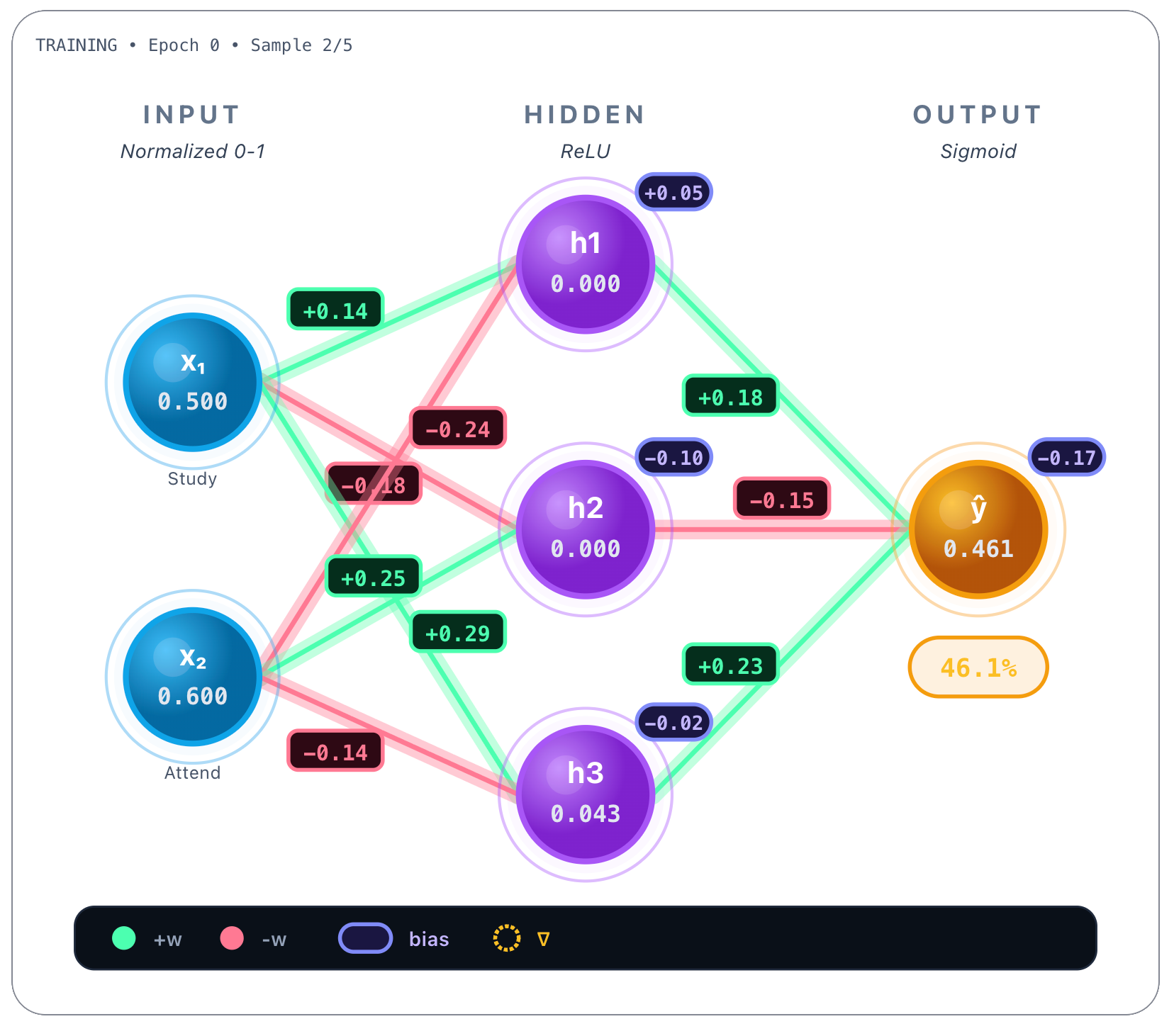
If you watch closely and compare with the weights in the beginning, they’ve changed! Each weight was updated in proportion to how much it contributed to the error. Active neurons update their weights, inactive neurons remain unchanged, and the model moves step by step toward lower loss.
And from here on the network would continue training and would iterate on all the available samples, sometimes more than once, that is, more than 1 epoch.
In theory, gradient descent computes the gradient using the entire training dataset. In practice, this is computationally expensive. Stochastic Gradient Descent (SGD) approximates the true gradient by computing it on a small random subset of the data. If you have a million points as training dataset, you would pick a batch size, let’s say 128. Then it would pick 128 samples randomly from the entire dataset (that’s why it’s called stochastic) and average them. Only then it would update the weights. This introduces noise into the optimization process, but dramatically speeds up training and often improves generalization. Most modern neural networks are trained using mini-batch SGD or adaptive variants such as Adam.
Well and this is it for Part 1. This post about LLM’s from scratch doesn’t have a lot of LLM specifics really, but these basic ANN building blocks are crucial for understanding what lies ahead. Next time we will do a deep dive on what kind of ANN’s LLM’s are built on and how are they effectively trained.
Until next time!