
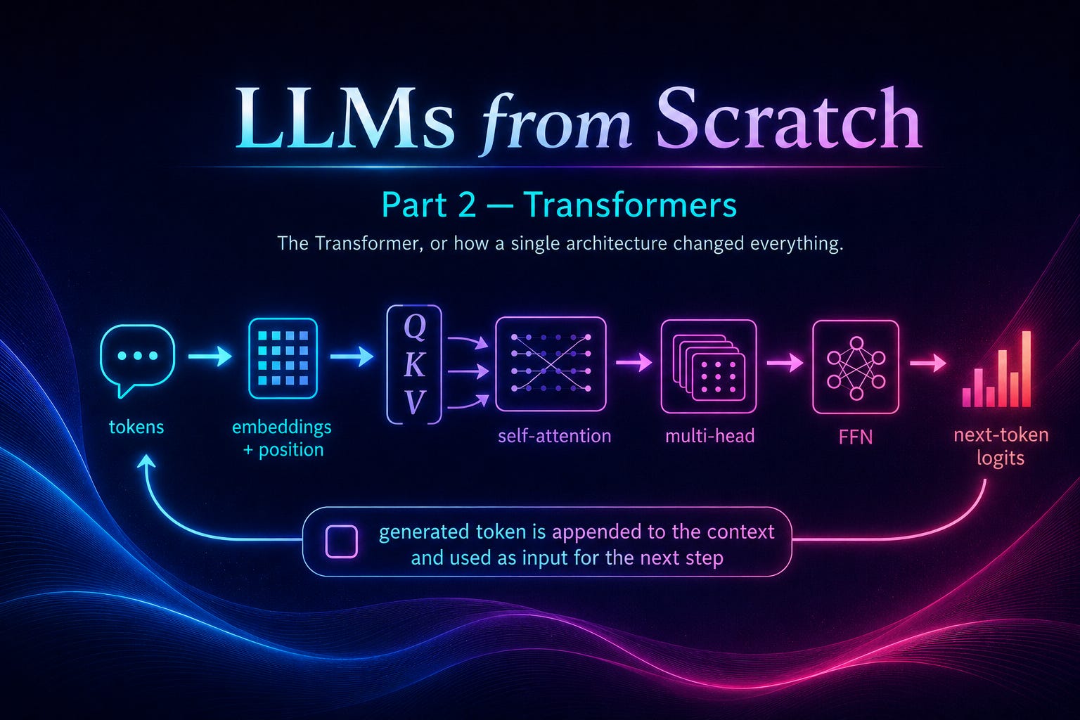
Large Language Models from scratch - Part 2
The Transformer, or how a single architecture changed everything.

In Part 1 we built a neural network from the ground up. We saw how neurons perform linear calculations, how activation functions introduce non-linearity, how the forward pass produces a prediction, and how backpropagation and gradient descent iteratively adjust every weight in the network to minimize the loss. We trained a small network to predict whether a student would pass or fail an exam based on study hours and class attendance. The math was simple. The principles were clear.
Now it’s time to go deeper. Much deeper.
What we built in Part 1 has a name. A network where every neuron in one layer is connected to every neuron in the next layer, where information flows strictly in one direction from input to output, with no loops and no memory — that’s called a Multi-Layer Perceptron, or MLP. The name traces back to Frank Rosenblatt’s Perceptron from 1958, which was a single artificial neuron that could learn to classify inputs into two categories. A single perceptron is just one neuron: it takes inputs, multiplies them by weights, adds a bias, applies an activation function, and produces an output. Stack multiple perceptrons in layers — an input layer, one or more hidden layers, an output layer — connect every neuron to every neuron in the adjacent layer, and you get a multi-layer perceptron. You’ll also encounter the terms “fully connected” or “dense” network, which mean the same thing.
MLPs are remarkably powerful in a theoretical sense. There’s a result called the Universal Approximation Theorem that says an MLP with a single hidden layer containing enough neurons can approximate any continuous function to arbitrary precision. In principle, given enough neurons and enough data, an MLP can learn anything.
But in practice, MLPs have a fundamental structural limitation: they take a fixed-size input and produce a fixed-size output, and they have absolutely no concept of order. When our student-exam network received (study_hours, attendance) as input, it didn’t matter which feature was “first” or “second” — those are just positions in a vector. There’s no temporal relationship, no sequence, no notion of “this came before that.”
This might seem like a minor issue, but it’s actually a devastating one when it comes to language. Consider two sentences:
“The dog bit the man” and “The man bit the dog”
Same words. Completely different meanings. The meaning lives in the order. An MLP that receives these words as a bag of features — ignoring position — would see them as identical. And even if we encoded position somehow, we’d face another problem: sentences have variable length. “Hi” is one token. “The quick brown fox jumps over the lazy dog” is nine. An MLP requires a fixed input dimension set at design time. Language simply doesn’t work that way.
This is the crack that opens the door to everything that follows.
I. The Road to the Transformer
The history of neural networks applied to language is essentially the history of trying to solve the sequence problem: how do you build a network that can process inputs of variable length, where the order of elements matters, and where elements far apart in the sequence can influence each other’s meaning?
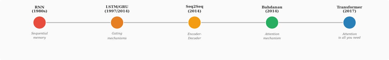
Recurrent Neural Networks (RNNs)
The first serious attempt was the Recurrent Neural Network. The idea, dating back to the 1980s, was elegant: give the network a form of memory. Instead of processing the entire input at once, an RNN processes it one element at a time, maintaining a hidden state that acts as a rolling summary of everything it has seen so far.
At each time step *t*, the RNN takes two inputs: the current element xtx_t xt (say, a word) and the previous hidden state ht−1h_{t-1} ht−1 (the memory of everything before). It combines them to produce a new hidden state:
Where Wh and Wx are weight matrices and α is an activation function (typically tanh). The hidden state ht is then both the output for this step and the memory carried forward to the next step.
This is clever. The network can handle sequences of any length because it processes them step by step. Word order is preserved because the hidden state accumulates information in the order it arrives. And in theory, information from the very first word can influence the processing of the very last word, because it’s encoded (however faintly) in the hidden state that gets passed forward at every step.
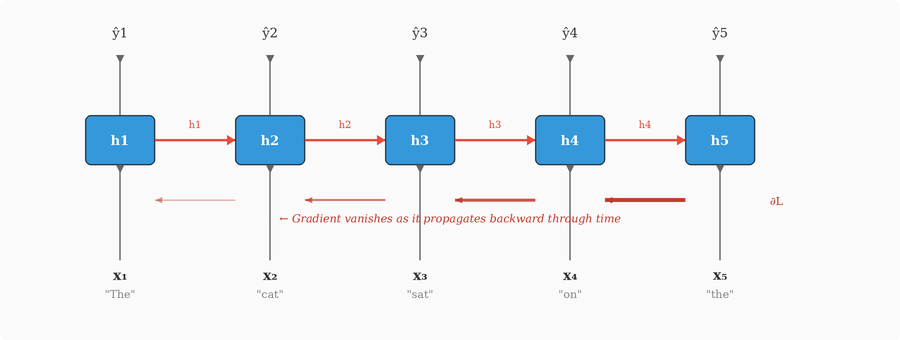
In practice, though, there’s a fatal problem: the vanishing gradient.
Remember how backpropagation works. We compute the loss at the output, then trace the chain of derivatives backward through the network to figure out how each weight contributed to the error. In an RNN, the chain goes backward through *time* — from the last word, through the second-to-last, through the one before that, all the way back to the first word. At each time step, the gradient gets multiplied by the weight matrix Wh. Here’s the problem: when you repeatedly multiply by the same matrix, the result tends to either shrink toward zero or explode toward infinity — depending on whether the matrix, loosely speaking, “contracts” or “expands” the vectors it’s applied to. (There’s a precise way to characterize this using a concept called *eigenvalues*, which we’ll explore properly later when we discuss residual connections.) In most practical cases, Wh is slightly contractive, so the gradient shrinks exponentially with each step. By the time it reaches words 20, 50, or 100 steps back, the gradient is effectively zero. The network can’t learn long-range dependencies because the error signal vanishes before it reaches the weights that need updating.
There’s also the opposite problem: if the eigenvalues are greater than 1, the gradients explode, growing exponentially and causing numerical instability. Gradient clipping can mitigate this, but the fundamental issue remains: vanilla RNNs struggle with sequences longer than about 10-20 elements.
LSTMs and GRUs
In 1997, Sepp Hochreiter and Jürgen Schmidhuber proposed the Long Short-Term Memory (LSTM) network, specifically designed to address the vanishing gradient problem. The key innovation was the introduction of gating mechanisms — learned switches that control what information to keep, what to forget, and what to output.
An LSTM cell maintains two kinds of state: a hidden state hth_t ht (like a regular RNN) and a cell state CtC_t Ct, which acts as a long-term memory highway. The cell state runs through time with minimal interference — information can flow along it unchanged unless a gate explicitly decides to modify it. This is the crucial insight: by providing a path where gradients can flow without being multiplied by weight matrices at every step, LSTMs allow error signals to propagate much further back in time.
The three gates are:
Forget gate: decides what information from the previous cell state to discard
Input gate: decides what new information to write into the cell state
Output gate: decides what part of the cell state to expose as the hidden state
The GRU (Gated Recurrent Unit), proposed in 2014 by Kyunghyun Cho, simplified the LSTM by combining the forget and input gates into a single “update gate” and merging the cell state and hidden state. It often performs comparably to LSTMs with fewer parameters.
Both LSTMs and GRUs dramatically improved the ability to model longer sequences, and they dominated NLP for years. But they still share a fundamental limitation inherited from the RNN paradigm: they process sequences one step at a time. Each hidden state depends on the previous one, creating a strict sequential dependency. This means:
No parallelism during training: you must compute h1h_1 h1 before h2h_2 h2, h2h_2 h2 before h3h_3 h3, and so on. On modern GPUs, which are massively parallel processors, this sequential bottleneck is extremely expensive.
The bottleneck problem persists: even with gates, there’s a practical limit to how much information can be compressed into a fixed-size hidden state vector. For very long sequences, early information still degrades.
Seq2Seq and the Encoder-Decoder Paradigm
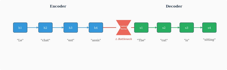
A major milestone came with the sequence-to-sequence (Seq2Seq) model, popularized around 2014 for machine translation. The idea was to chain two RNNs (typically LSTMs) together:
An encoder RNN reads the entire input sequence (say, a French sentence) one token at a time and compresses it into a single hidden state vector — the “context vector.”
A decoder RNN takes that context vector and generates the output sequence (the English translation) one token at a time.
This was a breakthrough for translation and other sequence-to-sequence tasks, but it had a glaring weakness: the entire meaning of the input sequence, no matter how long, had to be squeezed into a single fixed-size vector. That context vector was a bottleneck. For short sentences it worked reasonably well. For longer sentences, critical information inevitably got lost.
The Birth of Attention (Bahdanau, 2014)
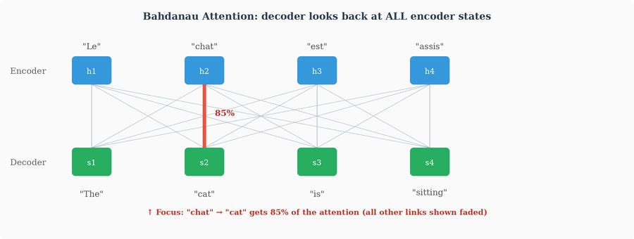
Dzmitry Bahdanau, Kyunghyun Cho, and Yoshua Bengio proposed a solution in their landmark 2014 paper: instead of forcing the decoder to rely on a single compressed context vector, let the decoder look back at all the encoder’s hidden states and decide which ones are most relevant at each decoding step.
This is the attention mechanism in its original form. At each step of decoding, the model computes a set of “attention weights” — one for each position in the input sequence — that say “how much should I focus on this part of the input right now?” These weights are used to create a weighted combination of all encoder hidden states, producing a custom context vector for each decoding step.
The intuition is natural. When a human translator is generating the English word “cat,” they focus on the French word “chat,” not on the article “le” or the period at the end of the sentence. The model learns to do the same thing: focus on what’s relevant, ignore what’s not, and the notion of “relevant” changes with each output token.
Bahdanau attention transformed the field. Translation quality improved significantly, especially for long sentences. But perhaps more importantly, it introduced an idea that would prove far more powerful than anyone initially realized: the notion that a network can learn to dynamically route information based on content, rather than relying on fixed connectivity patterns.
“Attention Is All You Need” (Vaswani et 2017)
By 2017, a group of researchers at Google — Ashish Vaswani, Noam Shazeer, Niki Parmar, Jakob Uszkoreit, Llion Jones, Aidan Gomez, Łukasz Kaiser, and Illia Polosukhin — asked a radical question: if the attention mechanism is doing the heavy lifting, why keep the recurrent structure at all?
Their paper, “Attention Is All You Need,” proposed the Transformer: an architecture that dispenses entirely with recurrence and convolutions, relying solely on attention mechanisms and feedforward networks. The results were striking — not only did the Transformer match or exceed the performance of the best RNN-based models, it was dramatically faster to train because it could process all positions in a sequence in parallel.
This wasn’t just an incremental improvement. It was a paradigm shift. Within a few years, virtually every state-of-the-art language model would be based on the Transformer architecture. BERT, GPT, T5, LLaMA, Claude — all Transformers. The architecture proved so versatile that it spread beyond language into vision (ViT), protein structure prediction (AlphaFold 2), music generation, robotics, and more.
Let’s now understand it completely.
II. Embeddings
Before we can walk through the Transformer, we need to understand one of the most important concepts in all of deep learning: embeddings. We touched on the idea that neural networks work with numbers, not words. But the question of how words become numbers, and what those numbers mean, is deeper and more beautiful than it first appears.
The Problem: Words Are Discrete
A neural network performs multiplications and additions. It works with continuous numbers — floating point values that can be added, multiplied, and differentiated. But language is discrete. The word “cat” isn’t a number. It’s a symbol from a finite vocabulary. You can’t meaningfully multiply “cat” by 0.7 or compute the gradient of “cat” with respect to anything.
The most naive approach to converting words into numbers is one-hot encoding. If your vocabulary has 50,000 words, you represent each word as a vector of length 50,000 where exactly one position is 1 and all others are 0. The word “cat” might be:
with the 1 at position 3,742 (wherever “cat” falls in the vocabulary).
This technically works, but it has serious problems:
Dimensionality: each vector has 50,000 dimensions. For a vocabulary of 100,000 tokens, each word is a 100,000-dimensional vector. This is wasteful and computationally expensive.
Sparsity: each vector is 99.998% zeros. Almost all the information is “this is not the word.”
No notion of similarity: in one-hot space, “cat” is exactly as far from “kitten” as it is from “democracy” or “earthquake.” Every word is equidistant from every other word. The representation captures no semantic relationships whatsoever.
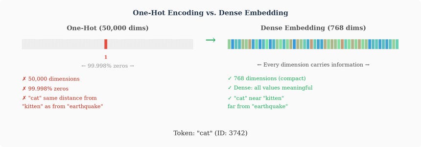
We need something better: a way to represent words as dense, low-dimensional vectors where similar words are near each other and dissimilar words are far apart.
The Embedding Matrix
The solution is an embedding matrix, and it’s much simpler than it sounds. It’s a matrix with shape (vocabulary_size × d_model), where d_model is the dimensionality of the embedding space (a hyperparameter we choose — common values are 768, 1024, 4096, or higher).
Each row of this matrix corresponds to one token in the vocabulary. Row 0 is the vector for token 0, row 3,742 is the vector for “cat,” and so on. To “embed” a word, you simply look up its row. That’s it. The embedding operation is a table lookup:
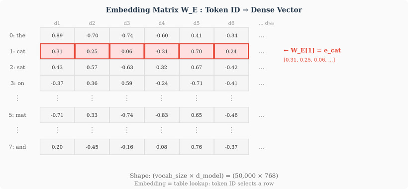
Go to row ii i, pull out the vector. No computation — just a memory access, like reading array[3].
You might wonder: how does a discrete index lookup — something that feels more like a database query than a mathematical operation — fit into a framework built entirely on differentiable matrix operations? Gradients need smooth, continuous functions, not integer indexing. The answer is that you *could* express the same lookup as a matrix multiplication using a one-hot vector. If x is a one-hot vector (all zeros except a 1 at position i, then:
The matrix multiplication with a one-hot vector simply selects row i. But nobody actually constructs the one-hot vector or performs this multiplication — it would be exactly the wasteful, sparse, high-dimensional operation we just argued against. The one-hot formulation exists purely to prove that the lookup is mathematically equivalent to a differentiable operation, which means gradients can flow through it during backpropagation. In practice, the embedding is implemented as a direct index: give me row ii i of the matrix. PyTorch’s nn.Embedding does exactly this.
So “cat” goes from a sparse 50,000-dimensional vector to a dense vector of, say, 768 dimensions. Something like:
These 768 numbers are the model’s understanding of the word “cat.” But here’s the crucial question: where do these numbers come from?
Where Does the Embedding Matrix Live in the Model?
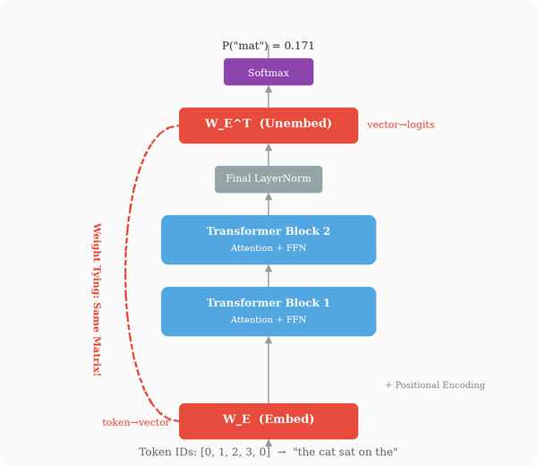
Before answering that, let’s place this matrix in the overall architecture. In a decoder-only LLM, the embedding matrix sits right at the input of the network — the first learned component a token encounters after tokenization. The input pipeline is:
Raw text → tokenizer → sequence of integer token IDs
Each token ID indexes into the embedding matrix to retrieve its embedding vector
Positional information is added (sinusoidal encoding, or RoPE applied inside attention)
The resulting vectors enter the first Transformer block
That’s the input side. But there’s a symmetric situation at the output. After all N Transformer blocks, the final vector at each position passes through an output projection matrix Whead (also called the “unembedding” or “LM head”) that maps from dmodel back to vocabulary space, producing one raw score per token in the vocabulary. These raw scores are called logits — a term borrowed from statistics that simply means "unnormalized scores before they're converted to probabilities." A logit can be any real number: positive, negative, or zero. By itself, a logit of 2.7 doesn't mean much — it only becomes meaningful once we compare it against all the other logits. That comparison happens via the softmax function, which converts the full vector of logits into a probability distribution (all values between 0 and 1, summing to 1). The token with the highest logit gets the highest probability.
Here’s the interesting part: in many modern LLMs, the output projection Whead is the same matrix as the input embedding matrix — specifically, its transpose. This technique is called weight tying (or “tied embeddings”). When weight tying is used, the embedding matrix effectively lives at both ends of the network: it turns token IDs into vectors at the input, and it measures how closely the network’s final output vector matches each token’s embedding at the output. The same geometric structure serves both translation directions.
The intuition for why this works geometrically: if the embedding of “cat” points in a certain direction in dmodel-dimensional space, then a final hidden vector that also points in that direction should have a high score for the token “cat.” That’s exactly what the transposed embedding matrix computes — the dot product between the output vector and each token’s embedding. So tying the matrices creates a consistent round-trip: the same geometry that converts tokens to vectors at the input is the geometry used to pick which token a vector is closest to at the output.
Weight tying is a design choice. It’s used in GPT-2 and many smaller models because it roughly halves the parameters of the embedding/output layer — which for large vocabularies can save hundreds of millions of parameters. Some larger models keep the matrices separate to give the output head more flexibility. Either way, the embedding matrix itself is a significant chunk of an LLM’s parameters: for a vocabulary of 128,000 tokens and dmodel=4096, the embedding matrix alone contains over 524 million parameters.
With the architectural placement clear, let’s return to the question of how these numbers come about.
How Embeddings Are Learned
The embedding matrix is initialized with random values. At the very beginning of training, the vector for “cat” is random noise — it encodes no meaning whatsoever. It’s no closer to “kitten” than to “democracy.”
But the embedding matrix is a parameter of the network, just like every weight matrix we saw in Part 1. It participates in the forward pass: the token’s embedding vector flows through the network, contributes to a prediction, and the prediction is compared against reality via the loss function. Then backpropagation computes the gradient of the loss with respect to every parameter — including the entries of the embedding matrix.
Let’s trace this concretely. Suppose the model is processing the sentence “The cat sat on the ___” and needs to predict the next word. It embeds each token, processes them through the network, and produces a probability distribution over the vocabulary. Let’s say it predicts “moon” with 30% probability and “mat” with 2% probability. But the true next word is “mat.”
The cross-entropy loss is high: the model was confident in the wrong answer. Backpropagation now computes
— how should the embedding vector for “cat” change to make this prediction less wrong? And :
— and so on for every token in the input. Gradient descent then nudges each embedding vector in the direction that reduces the loss.
Over billions of such updates across billions of sentences:
“cat” and “kitten” keep appearing in similar contexts (”The ___ purred,” “She petted the ___,” “The ___ chased the mouse”). Each time, the gradients push their embedding vectors in similar directions. Gradually, they drift closer together in the embedding space.
“cat” and “earthquake” almost never appear in similar contexts. Their gradients push them in unrelated directions. They drift apart, or simply never converge.
Subtler relationships emerge too. “king” and “queen” appear in similar contexts, but with systematic differences that correlate with gender. “walked” and “walking” appear in similar contexts but with differences that correlate with tense. The embedding space develops directions that correspond to these semantic properties.
This is worth pausing on. Nobody told the model that “king” and “queen” are related. Nobody defined “gender” as a concept. Nobody hand-crafted a taxonomy of semantic relationships. The only signal was the loss — billions of instances of “you predicted the wrong next word, here’s how wrong you were.” And from that signal alone, through the mechanics of gradient descent, the embedding matrix organized itself into a space where meaning has geometric structure.
The Geometry of Meaning
What does this geometric structure look like? Each embedding vector is a point in a high-dimensional space (768 dimensions, 4096 dimensions, or more). We can’t visualize these spaces directly, but we can reason about them using the tools of linear algebra.
Distance and similarity: two words with similar meanings have embedding vectors that are close together. “Similarity” is typically measured by cosine similarity — the cosine of the angle between two vectors:
A value of 1 means the vectors point in exactly the same direction (maximally similar). A value of 0 means they’re orthogonal (unrelated). A value of -1 means they point in opposite directions.
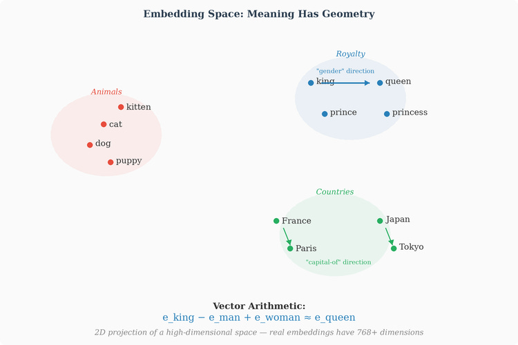
Linear substructures: the most famous finding from word embedding research (originally from Word2Vec, but it applies to all learned embeddings) is that semantic relationships correspond to directions in the embedding space. The classic example:
What this says is that there’s a direction in the embedding space that corresponds to the concept “male → female.” If you start at “king” and move in that direction, you arrive near “queen.” If you start at “uncle” and move in the same direction, you arrive near “aunt.” This direction wasn’t programmed — it emerged from the loss landscape because the systematic substitution patterns in language (contexts where “king” appears are similar to contexts where “queen” appears, modulo gender-correlated words) created gradient pressure that organized the space this way.
Similar directions encode other relationships: verb tense (”walking” − “walked” ≈ “swimming” − “swam”), country-capital relations (”France” − “Paris” ≈ “Japan” − “Tokyo”), and many more. These directions can’t easily be named or isolated in a single dimension. They’re distributed across many dimensions simultaneously — a concept might be partly encoded in dimension 47, partly in dimension 203, partly in dimension 651, combined in a way that only makes sense as a direction in the full high-dimensional space.
The Pressure of Many Directions
There’s a powerful image that makes the richness of embeddings click, and it’s worth spelling out explicitly because it justifies why embedding vectors carry so much concentrated meaning.
During training, each token in the vocabulary appears in countless different contexts. Consider the word “bank”:
“river bank” — gradients push its embedding toward concepts of geography, water, land, physical edges
“bank account” — gradients push toward finance, money, institutions, transactions
“blood bank” — gradients push toward medical, storage, biological concepts
“bank of clouds” — gradients push toward meteorology, collections, spatial aggregation
“bank the plane” — gradients push toward motion, aviation, tilting
“bank shot” — gradients push toward sports, angles, reflection
And hundreds or thousands of others
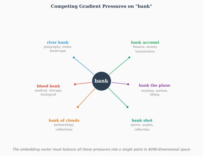
Every time “bank” appears in training, backpropagation computes how *this specific vector* — the single row in the embedding matrix indexed by the “bank” token — should change to reduce the prediction error for that context. And critically: **all these gradients flow back to the same vector**. The embedding for “bank” is updated by the finance contexts and the geography contexts and the aviation contexts and the sports contexts, all shaping the same 4096 numbers.
The vector cannot move in all these directions simultaneously at full strength. It has to find a single location in the high-dimensional space that, averaged over all the contexts in which this token appears, best serves the prediction task. This is an optimization problem with many competing objectives collapsed into one signal, and the solution the network converges on is a kind of balance — a vector that encodes a bit of every use of the word, weighted by frequency and by how much each context matters for prediction accuracy.
This is precisely where high dimensionality earns its keep. In a low-dimensional space — say 10 or 20 dimensions — these competing directional pressures would destructively interfere. Moving closer to “finance” would necessarily mean moving farther from “geography,” because there simply wouldn’t be enough independent directions to accommodate both. The vector would end up in some bland compromise that poorly serves any individual context.
In 4096 dimensions, there’s enough geometric room that “the finance direction” and “the geography direction” and “the aviation direction” can be nearly orthogonal to each other. The vector for “bank” can encode a substantial component along all of them simultaneously, because they point in different directions and don’t cancel out. The same vector can be near the finance cluster and near the geography cluster and near the aviation cluster — these are different directions in the space, and there’s room for all of them to coexist.
This is the concentrated richness of embeddings. Each vector is a dense multi-register pointer: it simultaneously encodes the word’s semantic neighbors along many different axes, because training pressure came from many different types of contexts. The embedding vector isn’t the word’s meaning in any single sense — it’s a compressed superposition of all the ways the word gets used, layered along nearly-orthogonal directions in a high-dimensional space. This is what the “richness” of a good embedding means: it carries many partial meanings at once, encoded along independent enough directions that downstream layers can pull out whichever one is relevant.
This framing also explains something that would otherwise be puzzling: why the Transformer’s contextual processing works. The raw embedding vector is an ambiguous superposition of all the word’s senses. But the Transformer’s attention layers can selectively read from specific directions. When processing “I deposited money at the bank,” the surrounding tokens (money, deposited) create an attention pattern that pulls the finance direction out of the bank vector and suppresses the geography direction. When processing “We sat on the bank of the river,” attention does the reverse. The embedding matrix stores all of it; the later layers disambiguate based on context.
By the time a vector has passed through 20, 40, or 80 Transformer blocks, it no longer represents “bank in general” — it represents “bank in this specific sentence, given the surrounding evidence.” The raw embedding was the full superposition; the network progressively collapses it toward the relevant sense. Hold this image — it explains why embeddings need to be rich, why dimensionality has to be high, and why the Transformer layers after the embedding layer are doing genuinely useful work rather than just copying information around.
Why So Many Dimensions?
Why 768 or 4096 dimensions? Why not 50 or 10?
Each dimension is a latent feature that the network discovered during training. You can’t point at dimension 347 and say “that’s the formality dimension.” The features are distributed, entangled, and not human-interpretable in isolation. But collectively, they need enough “room” to encode all the distinctions the model needs to make.
Think of it this way: the vocabulary might have 50,000 tokens. Each of those tokens has relationships with thousands of other tokens along dozens of semantic axes (topic, sentiment, formality, grammatical role, concreteness, temporal reference, and countless others). Compressing all of that into, say, 50 dimensions would force the model to reuse dimensions in conflicting ways — “dimension 12 encodes both formality and verb tense” — creating destructive interference. More dimensions give the model more room to represent distinct concepts along orthogonal directions without interference.
In practice, there’s a tradeoff: more dimensions mean more parameters, more computation, and more data needed to learn meaningful structure. The choice of embedding dimension is a design decision that balances model capacity against computational cost.
Embeddings Are Not Static
One crucial point: in modern Transformers, the embedding matrix produces the initial representation of each token, but that representation is then transformed by every subsequent layer of the network. After passing through 32 or 96 layers of attention and feedforward processing, the vector at position 5 is no longer just the embedding of the word that was originally at position 5. It has been enriched with contextual information from every other position in the sequence. The same word “bank” will have very different representations after processing in “river bank” versus “bank account.”
This is sometimes called contextual embeddings — the initial embedding captures the meaning of a word in isolation, but the Transformer layers progressively build a representation that captures the meaning of the word in this specific context. This is one of the reasons Transformer-based models dramatically outperform older approaches like Word2Vec, where each word had a single fixed embedding regardless of context.
Why Is This Matrix Called “Embeddings”?
Here’s a question worth pausing on, because it gets at something fundamental about how we think about these models — and it’s the same question that probably lurks in the back of your mind right now.
Think back to Part 1. Our student-exam MLP had several weight matrices — the weights connecting input to hidden layer, hidden layer to output. All of those matrices were learned through the same process: forward pass, compute loss, backpropagate, gradient descent. Mathematically, they all had identical status — just tensors of numbers being nudged by the chain rule.
The Transformer, as we’re about to see in the next section, contains many more learned matrices — it has weight matrices inside its attention mechanism, weight matrices inside the feedforward network (which is literally the same kind of MLP from Part 1), plus normalization parameters. All of them start random. All of them are shaped by the same loss. Yet we single out the embedding matrix and say its rows “mean” something. We say the vector for “cat” represents the meaning of “cat.” But we wouldn’t say the same thing about a row of one of the hidden-layer weight matrices from Part 1’s MLP. Why not?
And — to pose the sharpest version of the question — if we invented some extra matrix Winvented and inserted it somewhere in the architecture, it too would get learned weights, shaped by the loss. Would its rows “mean” something? What makes the embedding matrix semantically special compared to every other learned matrix?
This is a sharp question, and the answer illuminates something important. The status of a matrix as “semantic” — as carrying interpretable per-token meaning — doesn’t come from the math of how it’s updated. Every matrix is updated the same way. It comes from where the matrix sits in the architecture, and specifically what it is connected to.
The embedding matrix has one property that nothing else in the network has: it is indexed by discrete token identity. Row 3,742 of the embedding matrix is retrieved if and only if the token “cat” appears at an input position. Across the entire training corpus — across billions of training examples — every single gradient that flows back to row 3,742 originates from a context where “cat” specifically was being processed. That row accumulates, through sheer consistent association, everything the network ever had to know about “cat” in order to predict well.
No other matrix in the network has this property. Consider the weight matrices from Part 1’s student-exam MLP. The weights connecting the input layer to hidden neuron h1 were used for every student that passed through the network — they weren’t specific to any particular student. They encoded a transformation (how to combine study hours and attendance into a useful hidden feature), not a concept tied to a specific input. The same principle applies to every other weight matrix in a Transformer: they’re applied uniformly to whatever input flows through them, regardless of which token happens to sit there. They encode transformations — how to reshape an arbitrary input — not concepts tied to specific vocabulary items. They operate on already-processed representations, never having a clean one-to-one correspondence with discrete symbols.
The embedding matrix is the unique place in the network where a token’s identity is preserved as a retrievable address. It’s the only matrix where “row → specific token” is a stable mapping throughout training. And because of that, it’s the only place where per-token meaning can accumulate into a persistent vector.
Now, what about the thought experiment — what if we inserted an extra matrix Winvented between the embedding lookup and the first layer of the network? Would it learn meaningful representations?
It would learn something — every matrix does — but it wouldn’t be “embeddings” in the semantic sense. Here’s why: it would be applied uniformly to every input that flows through the network. It wouldn’t have per-token rows; it would be a single transformation. And mathematically, something even more telling happens: since the composition of two linear operations is itself a linear operation, such a matrix could be absorbed directly into the embedding matrix We. The “real” embedding matrix would still be the composite Winvented⋅We, because that’s what determines the final per-token vector that enters the first layer. The inserted matrix wouldn’t represent anything new; it would just redistribute the learned mapping across two matrices instead of one. In a sense, it would disappear into the embedding.
To get a second “embedding-like” matrix with its own distinct meaning, you’d need a second place in the architecture where discrete identity is preserved — a second kind of symbol that gets looked up by a distinct integer index. This is exactly what some architectures do: BERT has separate token embeddings, position embeddings, and segment embeddings, each indexed by a different discrete identity (token ID, absolute position, segment ID). Each of these is a legitimate “embedding” in the semantic sense — the rows of each matrix accumulate meaning for their respective kind of identity. They’re all embeddings, and they’re the only matrices in the network that qualify.
So what makes a matrix an embedding isn’t the fact that it’s learned — every matrix is learned. It’s the architectural privilege of being directly indexed by discrete identity. That’s the sole bridge between symbolic inputs and continuous computation, and the rows at that bridge are where symbolic meaning is anchored in the vector space. Every other matrix operates on what has already crossed the bridge.
This framing will become increasingly useful as we enter the next section and meet the Transformer’s many internal weight matrices. The Transformer contains dozens of learned matrices with names like K, Q, V — we’ll define each one carefully when we get there. But here’s the punchline you can take with you: they are all weight matrices in exactly the same sense as the weights in Part 1’s student-exam MLP. They start random. They’re updated by backpropagation. The loss is their only teacher. None of them are “embeddings” — they don’t have the architectural privilege of being indexed by discrete identity. What makes the Transformer powerful isn’t that it introduces some new type of parameter with new mathematical properties; it’s that it arranges ordinary weight matrices into a structure where useful computations are reachable via gradient descent.
Put another way: if you’re ever inclined to feel that embeddings are a fundamentally different kind of object from “just weights,” resist that intuition. They are just weights. What’s different is their position in the graph. And once you internalize that, the whole Transformer becomes conceptually simpler: it’s one big grid of learnable parameters, with a few of them (the embeddings) given the architectural privilege of being directly addressed by discrete tokens, and all the rest shaped by the loss into whatever useful transformations the architecture makes reachable.
III. The Transformer Architecture
We’re now ready to dissect the Transformer itself. We’ll go through every component of the architecture described in “Attention Is All You Need,” understanding not just what each piece does but why it’s there.
Tokenization
Before anything enters the model, raw text must be converted into a sequence of integers. This process is called tokenization, and the choices made here have surprisingly deep consequences.
The simplest approach would be to treat each word as a token. But this creates problems: the vocabulary would need to contain every word the model might ever encounter, including rare words, technical terms, names, and words from hundreds of languages. A word-level vocabulary would either be enormous (millions of entries) or would constantly encounter words it doesn’t recognize.
The opposite extreme — treating each character as a token — gives a tiny vocabulary (a few hundred entries) and never encounters unknown inputs, but sequences become very long and the model has to learn to assemble meaning from individual characters, which is inefficient.
Modern LLMs use a middle ground: subword tokenization. The two most common algorithms are Byte-Pair Encoding (BPE) and SentencePiece. The basic idea is:
Start with individual characters (or bytes) as the initial vocabulary.
Count which pairs of adjacent tokens appear most frequently in the training data.
Merge the most frequent pair into a single new token.
Repeat until the vocabulary reaches a target size (typically 32,000 to 128,000 tokens).
The result is a vocabulary where common words like “the” or “and” are single tokens, while rarer words are split into meaningful subunits. “Unhappiness” might tokenize as [”un”, “happiness”], and a very rare word like “defenestration” might become [”de”, “fen”, “est”, “ration”]. This gives the best of both worlds: a manageable vocabulary size, no unknown-word problem, and subword units that often correspond to meaningful morphological pieces.
Token Embeddings + Positional Information
Once text is tokenized into a sequence of integer IDs each token ID is used to look up its embedding vector from the embedding matrix, as we described in the previous section. This gives us a sequence of vectors:
Each ei has dimension dmodel (e.g., 4096).
But there’s a problem. The Transformer processes all positions in parallel, not sequentially like an RNN. This is a major advantage for speed, but it means the model has no inherent notion of word order. Without additional information, the Transformer would see “the cat sat on the mat” and “mat the on sat cat the” as identical — just a set of token embeddings with no positional structure.
We need to inject positional information somehow. The original “Attention Is All You Need” paper used sinusoidal positional encodings: fixed mathematical functions (sines and cosines of different frequencies) that generate a unique vector for each position, which is then added to the token embedding:
Where pi is the positional encoding for position i. The sinusoidal encoding was defined as:
Each dimension of the positional encoding uses a sinusoid with a different frequency. This has elegant properties: positions far apart have very different encodings, and the model can potentially learn to attend to relative positions because the difference between any two sinusoidal encodings depends only on their distance, not their absolute positions.
However, most modern LLMs have moved to a more sophisticated approach called Rotary Position Embeddings (RoPE), introduced by Jianlin Su et al. in 2021. RoPE is worth understanding because it’s used in LLaMA, Mistral, and most current open-source LLMs.
RoPE: Rotary Position Embeddings
The core idea behind RoPE is beautifully geometric: instead of adding a positional vector to the embedding, RoPE rotates the embedding vector by an angle proportional to its position.
To understand why rotation works, we need to think about what attention actually computes (we’ll see this fully in the next section, but the key point is relevant now). Attention computes the dot product between a query vector q at one position and a key vector k at another position. We want this dot product to depend on the relative distance between the two positions, not on their absolute positions.
RoPE achieves this by operating on pairs of dimensions. For a vector in d-dimensional space, RoPE groups the dimensions into d/2 pairs and applies a 2D rotation to each pair, where the rotation angle depends on the position:
Where m is the position index and θ_k = 10000^-2k/d sets a different rotation speed for each pair of dimensions.
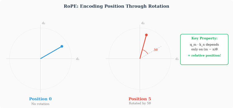
Why does this encode relative position? Because of a fundamental property of rotations: when you compute the dot product of two rotated vectors, the result depends only on the difference between their rotation angles, not on the angles themselves. If position m rotates by angle mθ and position n rotates by angle nθ, their dot product depends on (m-n)θ — the relative distance. This is exactly the property we want: the model’s ability to determine how far apart two tokens are doesn’t depend on where they sit in absolute terms, only on their relative distance from each other.
This has practical benefits too: since there’s no hard-coded maximum position, RoPE allows models to generalize (to some extent) to sequence lengths longer than those seen during training.
Self-Attention: The Core Mechanism
We’ve now embedded our tokens and encoded their positions. The sequence of vectors [x_1, x_2, ..., x_n] is ready to enter the Transformer’s core: the self-attention mechanism.
The fundamental question that attention answers is: for each token in the sequence, which other tokens should it pay attention to, and how much?
Consider the sentence: “The animal didn’t cross the street because it was too tired.” What does “it” refer to? To the animal, not the street. A human understands this instantly because of contextual reasoning. The attention mechanism gives the model the same ability: when processing the token “it,” the model can learn to attend strongly to “animal” and weakly to “street,” effectively resolving the reference.
Queries, Keys, and Values
The attention mechanism operates through three sets of vectors called queries, keys, and values. The metaphor is a soft dictionary lookup:
The query is what a token is “looking for” — what kind of information does it need?
The key is what a token “advertises” — what kind of information does it contain?
The value is what a token “gives” — the actual content it contributes when attended to.
For each input vector x_i, the model computes three vectors by multiplying with three separate learned weight matrices:
Where W_Q, W_K, and W_V are matrices of shape (d_model × d_k) for queries and keys, and (d_model × d_v) for values. These matrices are learned parameters — they start random and are shaped by gradient descent, just like the embedding matrix, just like every weight in the network. The loss is the only signal, and from it the model discovers what kinds of queries to form, what keys to advertise, and what values to pass along.
Why Not Just Use the Raw Vectors Directly?
This deserves a careful answer, because there’s an obvious simpler alternative: just compute dot products between the raw input vectors x_i and x_j to measure similarity, then use those as attention weights to mix the raw vectors. No W_Q, no W_K, no W_V — just raw similarity between embeddings. Why introduce three extra learned matrices?
The answer has several layers.
First: what a token needs to look for is not the same as what it contains. Consider the word “it” in “The animal didn’t cross the street because it was too tired.” The embedding vector for “it” encodes what “it” is — a pronoun, third person, singular. But what “it” needs — the information it must retrieve to be useful — is entirely different: it needs to find its antecedent, “animal.” The query for “it” should be something like “I’m looking for a noun that could be my referent,” while the key for “animal” should be something like “I’m a noun that could be someone’s referent.” These are fundamentally different roles, and a single raw vector can’t play both roles simultaneously. W_Q transforms the raw vector into a “what am I looking for?” representation, while W_K transforms the same raw vector into a “what do I advertise?” representation. These two projections allow the same token to ask one kind of question and answer a different kind.
Second: what you retrieve should be different from what you match on. Even once the attention pattern is decided — “position 6 should attend strongly to position 1” — the information that flows from position 1 to position 6 shouldn’t just be position 1’s raw embedding or its key. The key’s job was to get selected; the value’s job is to contribute useful content once selected. For example, the key for “animal” might encode “I am a concrete noun, animate, singular” (the properties that make it match the query from “it”), but the value for “animal” might encode the specific semantic content that “it” needs for downstream processing — information about what kind of entity it is, its role in the sentence, etc. W_V creates this separate “payload” that gets transmitted once a match is made.
Third: without projections, attention would be symmetric and context-blind. The dot product of raw vectors x_i · x_j is symmetric — it equals x_j · x_i. This means token A would attend to token B exactly as much as B attends to A. But in language, relationships are rarely symmetric: “it” should attend strongly to “animal,” but “animal” shouldn’t particularly need to attend to “it” at all. The separate W_Q and W_K matrices break this symmetry: q_i · k_j ≠ q_j · k_i in general, because different matrices are applied on each side.
Fourth: projections give the model learnable control over what matters. Raw embedding similarity is fixed by the embedding matrix. But attention needs to change its behavior at every layer. In block 3, attention might need to group tokens by syntactic role. In block 15, it might need to group them by semantic topic. In block 30, it might need to match questions with their answers. Each block has its own W_Q, W_K, W_V matrices, so each block can define “similarity” differently. The raw embeddings are the same everywhere; the projections give each layer its own notion of relevance.
In summary: W_Q, W_K, and W_V decouple three fundamentally different roles — asking, advertising, and contributing — that a single vector cannot serve simultaneously. Without them, attention would be a rigid, symmetric similarity measure over fixed representations. With them, attention becomes a flexible, asymmetric, learnable routing mechanism that can implement different information-flow patterns at every layer of the network.
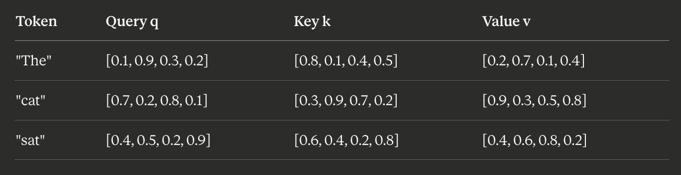
Let’s walk through a concrete example with small dimensions to build intuition. Suppose we have a 3-token sequence and d_k = d_v = 4 (real models use 64 or 128, but the mechanics are identical).
After the linear projections, we have:
Scaled Dot-Product Attention
Now comes the core computation. For each pair of positions (i, j), we compute how much position i should attend to position j by taking the dot product of the query at position i with the key at position j:
The dot product measures how aligned two vectors are — if the query and key point in similar directions, the score is high, meaning “this token has relevant information for what I’m looking for.” If they’re orthogonal, the score is zero, meaning “not relevant.”
For our 3-token example, we compute all pairwise dot products to form the attention score matrix:
Each row tells us: for this token’s query, how relevant is every other token’s key?
But before we turn these scores into weights, we scale them by dividing by √{d_k}:
Why? It’s about controlling variance. When d_k is large (say 64 or 128), the dot product of two random vectors tends to have a large magnitude — specifically, its variance grows proportionally to d_k. Large input values to the softmax function push it into regions where the gradient is extremely small (softmax saturates — one value dominates and all others are near zero). This makes learning difficult. Dividing by √{d_k} normalizes the variance back to 1, keeping the softmax in a well-behaved regime where gradients can flow.
Now we apply softmax to each row of the scaled score matrix:
Softmax converts each row of raw scores into a probability distribution — the values are all positive and sum to 1. Each row A[i, :] now contains the attention weights for position i: how much attention does position i pay to every other position?
Finally, we compute the output by using these attention weights to take a weighted sum of the value vectors:
In matrix form:
The output for each position is a blend of all value vectors, weighted by how relevant each position’s key was to this position’s query. If position i attends strongly to position j (high A[i,j]), then position j’s value vector contributes heavily to position i’s output. If the attention weight is near zero, that position’s value barely contributes.
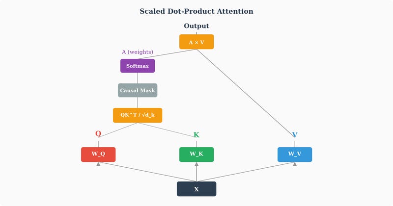
This is the complete attention mechanism. And notice something crucial: every component — W_Q, W_K, W_V — is a learned weight matrix. The model discovers, through gradient descent against the loss, what queries to ask, what keys to advertise, and what values to pass. Nobody programs the model to resolve coreferences or track syntactic dependencies. The loss function says “you predicted the wrong next word,” and backprop shapes these matrices until the attention patterns that emerge are the ones that best reduce prediction error.
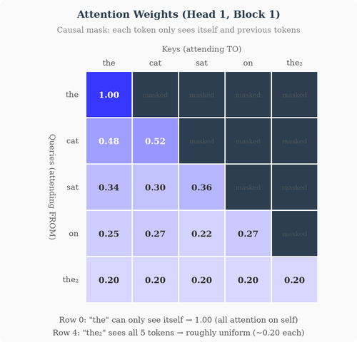
Causal (Masked) Attention
In the original Transformer (designed for translation), the encoder uses bidirectional attention — each token can attend to every other token in the sequence, including tokens that come after it. This makes sense for understanding input: to comprehend the meaning of a word, you need the full context.
But for generation — predicting the next token — you cannot look at future tokens. When the model is trying to predict what comes after “The cat sat on the,” it can’t peek at the answer. This would be cheating during training, and during inference the future tokens simply don’t exist yet.
The solution is a causal mask (also called a “look-ahead mask”): a lower-triangular matrix of ones and zeros (or equivalently, negative infinities and zeros) that is added to the attention scores before softmax:
Adding -∞ to a score before softmax effectively sets that attention weight to zero — position i is prevented from attending to any position j > i. Token 1 can only see itself. Token 2 can see tokens 1 and 2. Token 3 can see tokens 1, 2, and 3. And so on.
This is why decoder-based models (GPT-style) are called autoregressive: they generate text one token at a time, each token conditioned only on the tokens that came before it.
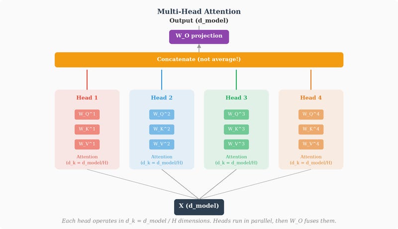
Multi-Head Attention
A single attention operation computes one set of attention weights for each position. But a token might need to attend to different parts of the sequence for different reasons. “it” in our earlier example needs to attend to “animal” for coreference resolution, but it might also need to attend to “tired” to understand the predicate, and to “didn’t” to understand negation.
Multi-head attention addresses this by running multiple attention operations in parallel, each with its own learned W_Q, W_K, W_V matrices:
Each head has a reduced dimensionality: if d_model = 768 and we have h = 12 heads, each head operates in d_k = d_v = 768/12 = 64 dimensions. This is the crucial design choice. Each head doesn’t see the full 768-dimensional representation — it’s forced to work with only 64 dimensions. Head 1 operates in one 64-dimensional subspace, head 2 in a different 64-dimensional subspace, and so on.
This dimensional constraint is what forces the heads to develop different perspectives. If every head operated on the full 768 dimensions, they’d all be looking at the same information and solving the same optimization problem — different random initialization might give early diversity, but gradient descent would tend to push them toward similar solutions over training. By restricting each head to a small subspace, the architecture guarantees that each head must learn to form useful attention patterns from a different slice of the representation. Head 1 can only see features that live in its 64 dimensions. Head 2 can only see features in its own, different 64 dimensions. The diversity is structurally enforced, not hoped for.
There’s also a computational benefit: the total cost of H heads at d_k dimensions each equals the cost of a single head at the full d_model dimensions. You get multiple perspectives for the same price as one.
Why Not Just One Big Head?
It’s worth pausing on the tempting alternative: instead of H small heads, why not use a single head at the full d_model width and skip the splitting (and W_O) entirely? The first thing to notice is that this wouldn’t save anything. A single full-width head needs three d_model × d_model matrices — that’s 3 × d_model^2 parameters. Multi-head uses the same 3 × d_model^2 for all its Q/K/V projections combined, because stacking H matrices of width d_k = d_model/H side by side reconstructs a d_model × d_model matrix. Multi-head then adds W_O on top, so it’s actually slightly more expensive, not cheaper. Saving parameters was never the motivation — the total query/key/value capacity is identical either way.
The real reason is what a single head can and cannot do. No matter how wide you make it, one head produces exactly one set of attention weights per position — one softmax distribution over the sequence. And softmax is competitive: it sums to 1, so attending strongly to one token necessarily suppresses the others. But “it” in our example needs to look at “animal” (its referent) and “tired” (the predicate) and “didn’t” (negation) at the same time. A single distribution can’t point firmly in several directions at once — it’s forced into a blurry compromise. Widening the head gives it richer query and key vectors, but it still collapses them into a single softmax: same bottleneck, just higher-dimensional inputs. What you actually need is several independent attention patterns, and that is precisely what H heads provide — H separate softmaxes that don’t compete, later fused by W_O.
Seen this way, the dimensional slicing isn’t the goal; it’s the mechanism that lets you afford many attention patterns on a fixed budget. You have d_model “query dimensions” to spend, and H simply decides how many independent patterns you carve them into. The authors didn’t just guess at this — the original paper ran the ablation, reporting that a single head was about 0.9 BLEU worse than the multi-head configuration at the same total dimensionality, while using too many heads (each too thin to form discriminating dot products) also hurt quality. The H = 8, d_k = 64 region was the sweet spot: enough parallel patterns, each still wide enough to be sharp.
After all heads compute their outputs, the results are concatenated and passed through a final linear projection:
Where W_O is yet another learned weight matrix of shape (d_model × d_model) that blends the outputs of all heads back into the full d_model-dimensional space.
A Note on Implementation
Conceptually, each head has its own separate small W_Q, W_K, W_V matrices — and that’s the clearest way to think about it. But in actual PyTorch implementations, you’ll see something different: one large W_Q matrix of shape (d_model, d_model) that processes the input in a single matrix multiplication, and then the result is reshaped into H separate chunks of d_k dimensions. This produces identical numbers to the “separate small matrices” approach — stacking H matrices of shape (d_model, d_k) side by side gives one matrix of shape (d_model, d_model), and multiplying then slicing is the same as slicing then multiplying. The single large multiplication is just much faster on a GPU, which is optimized for big, regular operations. The “reshape” itself is free — no data is copied or moved, the GPU just reinterprets the same memory as having a different shape.
Why Do We Need W_O After Concatenation?
At this point you might ask: isn’t the concatenated vector already the right shape? If each head outputs a vector of dimension d_v = d_model/H, and we concatenate H of them, we get a vector of dimension d_model. That’s the same dimension the rest of the network expects. Why not just use the concatenated vector directly and skip the extra matrix?
The concatenated vector has a structural problem: it’s compartmentalized. Dimensions 0 through d_v - 1 came entirely from head 1. Dimensions d_v through 2d_v - 1 came entirely from head 2. And so on. There’s no mixing between heads. Whatever head 1 computed sits in its own section, whatever head 2 computed sits in its section, and the two sections never interact.
But the downstream layers — the residual connection, the FFN, the next block’s attention — expect a single unified representation at each position, not a partitioned one. The next block’s W_Q matrix, for instance, will multiply the entire d_model-dimensional vector to produce a new query. If that query needs to combine information from something head 1 discovered (say, syntactic structure) with something head 2 discovered (say, semantic similarity), it would need to reach into both compartments of the concatenated vector simultaneously. Without W_O, the only way to mix these compartments is to leave it to the next layer’s matrices, which means the network has to “waste” some of its capacity in those matrices just to undo the compartmentalization from the previous layer.
W_O solves this by performing a cross-head mixing immediately after concatenation. It’s a full (d_model × d_model) matrix, so every dimension of its output can be a weighted combination of every dimension of its input — mixing head 1’s contributions with head 2’s, head 3’s, and so on. This lets the network produce a coherent, unified representation that combines the best insights from all heads, rather than passing along a segmented structure and hoping downstream layers sort it out.
Think of it this way: the multiple heads are like a panel of experts who each analyzed the sequence from their own perspective. Concatenation puts their reports side by side on a desk. W_O is the decision-maker who reads all the reports and writes a single, integrated summary. That summary is what the rest of the network acts on.
W_O is also a learned parameter — shaped by the loss just like everything else — so the network discovers the best way to fuse head outputs for the prediction task. In practice, trained W_O matrices often show interesting structure: some output dimensions draw heavily from one specific head, others blend several heads, reflecting the fact that different aspects of the final representation benefit from different combinations of the heads’ outputs.
Different heads learn to specialize in different things. Research on trained Transformers has found heads that track syntactic dependencies (subject-verb agreement), heads that handle coreference (pronoun resolution), heads that focus on nearby tokens (local context), and heads that attend to distant tokens (long-range dependencies). This specialization isn’t programmed — it emerges from the loss function, because having diverse attention patterns leads to better predictions.
The Feedforward Network (FFN)
After the multi-head attention layer, each position’s vector passes through a position-wise feedforward network. And here’s where we come full circle to Part 1, because this feedforward network is nothing more and nothing less than an MLP — the exact same kind of network we built from scratch.
Remember our student-exam network? It had an input layer (2 neurons: study hours, attendance), a hidden layer (3 neurons), and an output layer (1 neuron). Each layer was fully connected to the next. That was an MLP. The FFN inside each Transformer block is the same thing, just with different dimensions:
Input layer: the d_model-dimensional vector at a single position (e.g., 4096 dimensions)
Hidden layer: d_ff neurons (e.g., 16384 = 4 × 4096)
Output layer: back to d_model dimensions (4096)
That’s it. The entire example from Part 1 — the student pass/fail predictor with its weights, biases, linear combinations, activation functions, and backpropagation — is just a small component inside a single Transformer block. Every Transformer block contains one of these MLPs. A 32-block Transformer contains 32 separate MLPs (each with its own weights).
Let’s be explicit about the connection. In Part 1, a single neuron computed:
The FFN's first layer does the exact same thing, just for all neurons at once using matrix notation:
Each row of W₁ is the weight vector for one neuron in the hidden layer. The matrix multiplication computes all the linear combinations simultaneously. Then the activation function is applied element-wise:
And the second layer contracts back:
Written in one line:
Where W₁ has shape (d_model × d_ff) and W₂ has shape (d_ff × d_model). Typically d_ff = 4 × d_model, so the FFN expands the representation to a wider space, applies the non-linearity, and then projects it back down.
Why is it necessary to “Expand and Contract” ?
The term “expand and contract” describes what happens dimensionally, but let’s trace what this means for the information flowing through.
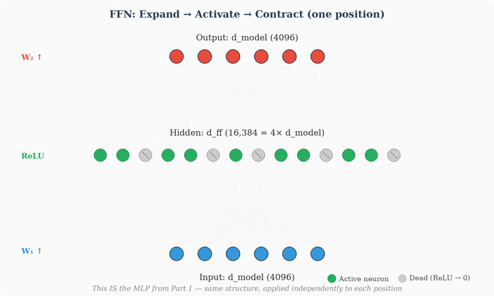
When a 4096-dimensional vector enters W₁ and becomes a 16384-dimensional vector, the representation has been projected into a much wider space. Each of these 16384 dimensions is a learned feature detector — a specific linear combination of the input’s 4096 dimensions, followed by a nonlinear activation. Some of these feature detectors might activate (produce a non-zero value) for inputs related to animals, others for inputs related to past tense, others for inputs that look like the start of a list. The wider space gives the network 16384 “slots” to check for different patterns.
The activation function then decides which of these feature detectors “fire.” With ReLU, any dimension that computed a negative value gets zeroed out. Only the relevant features survive. This is sparse activation — in practice, at any given position, most of the 16384 neurons are inactive (zero). The activation function selects which features are relevant for this particular input.
Then W₂ takes the surviving (non-zero) activations and projects them back to 4096 dimensions. Each column of W₂ is the “contribution” that one hidden neuron makes to the output. The second matrix effectively says: “given that these particular features activated, here’s how to update the representation.” It combines the active features’ contributions into a coherent d_model-dimensional update.
The expand-then-contract pattern is like this: the first matrix asks 16384 yes/no questions about the input (expansion), the activation function selects the relevant answers (gating), and the second matrix synthesizes the relevant answers back into a compact representation (contraction).
Activation Function: GELU vs ReLU
GELU (Gaussian Error Linear Unit) has largely replaced ReLU in modern Transformers. Where ReLU hard-clips negative values to zero, GELU applies a smooth, probabilistic gating:
Where phi(x) is the cumulative distribution function of the standard normal distribution. Intuitively, GELU multiplies each value by the probability that a standard Gaussian random variable is less than that value. Small negative values are smoothly dampened rather than harshly zeroed, which empirically leads to better training dynamics.
Why Is the FFN Needed At All?
Attention handles the mixing of information across positions — it lets each token gather relevant information from other tokens. But it doesn’t do much processing of that gathered information. The attention output at each position is a weighted average of value vectors, which is still a linear combination. Non-linear processing — the ability to compute complex functions of the gathered information — requires the FFN.
Think of it this way: attention is the “communication” step (tokens exchange information), and the FFN is the “thinking” step (each token independently processes what it received). Without the FFN, the Transformer would just be stacking linear operations on top of linear operations (since the attention mechanism is fundamentally a weighted average, which is linear in the values). The FFN’s activation function is what introduces genuine non-linearity, giving each block the computational power to learn complex transformations.
The FFN as a Key-Value Memory
Recent research has suggested an elegant interpretation: the FFN layers act as key-value memories. The first matrix W₁ maps the input to a set of “keys” in the wider space, the activation function selects which keys are active, and the second matrix W₂ retrieves the associated “values.” In this view, each neuron in the wider layer stores a piece of knowledge, and the input determines which pieces of knowledge are retrieved. This is why scaling up the FFN (making d_ff larger) tends to increase the amount of factual knowledge a model can store.
The FFN Is Applied Per-Position — Independently
One detail worth emphasizing: the FFN is applied independently to each position in the sequence, using the same weights for every position. Position 0’s vector goes through W₁ and W₂. Position 1’s vector goes through the same W₁ and W₂. Position 2 the same. They share weights but don’t interact — there’s no information flow between positions inside the FFN. All cross-position communication happens in the attention layer. The FFN is purely a per-position transformation.
This is different from the student-exam MLP in Part 1, where the entire input was fed in at once. Here, the FFN processes one position’s vector at a time (though in practice, for efficiency, all positions are batched through the same matrix multiplication simultaneously — the math is the same either way).
SwiGLU: The Modern FFN Variant
The FFN we described above — two matrices with an activation in between — is what the original Transformer paper used. But most modern LLMs, including LLaMA, Mistral, and their derivatives, use a modified version called SwiGLU (Swish-Gated Linear Unit), introduced by Noam Shazeer in 2020. Understanding this variant matters not just for comprehension but for practical work: if you ever fine-tune an LLM with techniques like LoRA, you’ll encounter the names of these matrices directly.
The standard FFN has two weight matrices:
W₁ expands from d_model to d_ff, ReLU activates, W₂ contracts back. Two matrices, one activation.
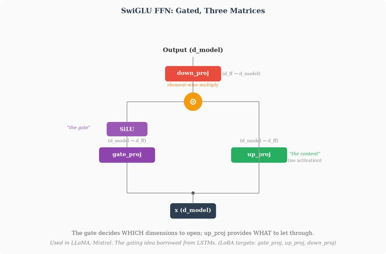
SwiGLU replaces this with three weight matrices and a gating mechanism:
Where ⊙ denotes element-wise multiplication — multiplying two vectors entry by entry. The three matrices have specific roles:
W_gate (the “gate projection”): projects from d_model to d_ff, then passes the result through SiLU (Sigmoid Linear Unit, also called “Swish”), a smooth activation function. SiLU is defined as SiLU(x) = x · sigmoid(x), which is similar to GELU but simpler to compute. The output of this path is a vector of gating values — numbers that determine how “open” each dimension is. Values near zero mean “block this dimension,” values near one mean “let it through.”
W_up (the “up projection”): also projects from d_model to d_ff, in parallel with the gate path. This produces the actual content — the information that might pass through. No activation function is applied here. This is the raw signal.
W_down (the “down projection”): projects from d_ff back to d_model. This is the contraction step, playing the same role as W₂ in the standard FFN.
The key difference from the standard FFN: instead of one matrix producing values that ReLU then hard-clips, two matrices collaborate. The gate path decides which dimensions to open (via SiLU), the up path provides what content to let through, and the element-wise multiplication combines them — only information that the gate “approves” survives. Then the down projection compresses the result back to d_model dimensions.
This is the same gating idea that made LSTMs effective — learned gates that control information flow — now applied inside the FFN. It gives the network finer-grained control over what information passes through, compared to ReLU’s blunt “positive values live, negative values die” approach. Empirically, SwiGLU produces better results than standard ReLU or GELU FFNs at the same parameter count.
There’s a practical consequence worth noting. The standard FFN has two weight matrices (W₁ and W₂), while SwiGLU has three (gate, up, down). To keep the total parameter count comparable, SwiGLU models typically use a smaller d_ff. For example, where a standard FFN might use d_ff = 4 × d_model, a SwiGLU FFN might use d_ff = 8/3 × d_model (roughly 2.67×). With three matrices at the smaller width, the total parameter count ends up similar to two matrices at the larger width.
Why this matters for fine-tuning: when you fine-tune a model using LoRA (Low-Rank Adaptation) or similar techniques, you select which weight matrices to apply adapters to. A typical LoRA configuration targets some or all of these matrices:
q_proj, k_proj, v_proj, o_proj — the four attention matrices (W_Q, W_K, W_V, W_O from the attention section)
gate_proj, up_proj, down_proj — the three SwiGLU FFN matrices
Now you know exactly what each of those names refers to. The attention projections are the Q/K/V matrices and the output projection we described in the attention section. The gate/up/down projections are the three FFN matrices we just described. Every learnable matrix in a modern Transformer block is covered by these seven names (plus the LayerNorm parameters, which are usually not targeted by LoRA because they’re small).
Mixture of Experts: Scaling the FFN Without Scaling Compute
Everything we’ve described so far is a dense Transformer — every parameter participates in every forward pass, for every token. But there’s an increasingly popular architectural variant that modifies the FFN specifically, leaving everything else untouched: Mixture of Experts (MoE).
The idea flows naturally from two observations we’ve already made. First, the FFN acts as a key-value memory — each neuron in the hidden layer stores a piece of knowledge, and the activation function selects which neurons fire. Second, only a fraction of neurons activate for any given input (the rest are zeroed by ReLU). So most of the FFN’s capacity is “dark” at any given moment. What if we leaned into that sparsity more aggressively?
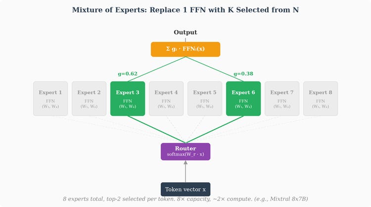
A MoE layer replaces the single FFN with multiple independent FFNs — typically 8, 16, or even 64 — called experts. Each expert is a complete FFN: its own W_1^(e), activation, W_2^(e), biases. Structurally identical to the FFN we described, just replicated several times with independent weights.
On top of the experts sits a small learned router network (also called a gating network) — typically a single linear layer followed by softmax — that takes each token’s vector as input and produces a probability distribution over the experts:
Where W_router has shape (d_model × n_experts) and g is a vector of n_experts probabilities saying “how relevant is each expert for this token?”
The key design choice is top-k routing: instead of running all experts, the router selects only the top k (typically k = 2) experts with the highest gating scores. Only those k experts run their forward pass for this token. The outputs of the selected experts are then combined as a weighted sum, using the gating scores as weights:
Everything else in the Transformer block stays exactly the same. The block becomes:
LayerNorm → Multi-Head Attention → Residual → LayerNorm → Router → top-k FFNs → Residual
Attention is unchanged. Residuals are unchanged. Normalization is unchanged. Only the FFN slot is swapped out.
Why does this matter? It decouples the model’s total knowledge capacity from its per-token compute cost. Consider Mixtral 8x7B, a well-known MoE model. It has 8 experts, each roughly the size of a 7B-parameter model’s FFN. The total parameter count is about 47 billion. But with top-2 routing, only 2 of the 8 experts run for any given token, so the active parameter count per token is about 13 billion. The model has the knowledge capacity of a ~47B dense model but the inference cost of a ~13B dense model. It gets the quality benefits of scale without the full computational price.
This connects directly to the “FFN as key-value memory” interpretation. A single FFN has a fixed number of memory slots (neurons in the hidden layer). If you want the model to know more facts, you need more slots, which means a bigger d_ff, which means more compute per token. MoE breaks this tradeoff: 8 experts means 8× the memory slots, but since only 2 run per token, the compute only doubles rather than octupling. Different experts can specialize in different domains of knowledge — one might activate for medical text, another for code, another for legal language — and the router learns which bank of knowledge is relevant for each token. The router itself is learned through the same loss and gradient descent process as everything else: it starts random, and the loss signal shapes it to route tokens to whichever experts reduce prediction error.
There are engineering subtleties we won’t dive deep into — load balancing (ensuring all experts get used, not just a few favorites), auxiliary losses (penalties that encourage balanced routing), and the communication overhead in distributed training (different experts may live on different GPUs). But architecturally, MoE is a clean substitution at the FFN level. If you understand the dense FFN, you understand MoE — it’s the same computation, replicated and gated.
Layer Normalization and Residual Connections
Two more components are essential for making deep Transformers trainable:
Residual connections (also called skip connections) add the input of a sub-layer directly to its output:
This looks like an innocuous formula — just adding two vectors. But it’s arguably the single most important structural innovation that makes deep Transformers trainable. Without residual connections, a 32-block Transformer would be practically impossible to train. With them, networks of 80 or even 128 blocks train reliably. Let’s understand why.
The Problem Without Residual Connections
Imagine a deep network without residual connections. Each block applies a transformation f to its input:
The output is the result of composing all these functions: f_N applied to f_{N-1} applied to ... applied to f_1 applied to x_0 — a long chain. During backpropagation, the chain rule tells us the gradient of the loss with respect to an early layer's parameters involves the product of all intermediate derivatives:
Each of those derivative terms is a Jacobian matrix. In Part 1, our network had scalar values flowing between neurons, so each derivative was just a single number. But in a Transformer, what flows between layers are vectors (4096-dimensional, say), and the derivative of a vector-valued function with respect to a vector input is a matrix, not a scalar. The Jacobian is simply that matrix: each entry tells us how much one particular output dimension changes when we nudge one particular input dimension. It’s the multi-dimensional generalization of the single-number derivative from Part 1.
In Part 1, we saw the chain rule multiplied through each layer’s derivatives — each was a scalar, and we multiplied scalars together. Here, the chain rule multiplies Jacobian matrices together. And just as a product of many small scalars (each less than 1) shrinks toward zero, a product of many matrices can shrink too — but the notion of “small” for a matrix is captured by its eigenvalues.
An eigenvalue is, informally, a number that tells you how much a matrix stretches or shrinks along a particular direction — but the eigenvalue itself is just a scalar, not a direction. The direction comes from its paired eigenvector. They always come together: every square matrix has a set of special vectors (called eigenvectors) along which the matrix acts like simple scalar multiplication instead of the usual rotation-and-scaling. The defining equation is Av = λ v: the matrix A applied to eigenvector v gives back the same vector v scaled by λ. The eigenvector v says which direction is special; the eigenvalue λ says what happens along that direction. If λ = 0.9, any component of a vector that lies along eigenvector v gets shrunk by 10% each time the matrix is applied. If λ = 1.1, that component grows by 10%. If λ = 1, it’s preserved exactly.
With that context: if these Jacobians typically have eigenvalues less than 1 (which is common — most learned transformations are slightly contractive), then multiplying 32 or 80 of them together gives a product that approaches zero exponentially fast:
The gradient that reaches the first block is essentially zero. The early layers receive no meaningful error signal, so they can’t learn. This is the vanishing gradient problem — the same phenomenon that plagued RNNs, now showing up in the depth dimension instead of the time dimension.
What Residual Connections Change
With a residual connection, each block computes:
This tiny change — adding the input back to the output — transforms the gradient picture entirely. Let's see why. Taking the derivative with respect to x_i:
Where I is the identity matrix — a square matrix with 1s on the diagonal and 0s everywhere else, which acts like the number 1 for matrices: multiplying any vector by I returns the same vector unchanged. This is the crucial difference. Without the residual, the derivative was just the Jacobian of the sub-layer — a matrix that might have small eigenvalues. With the residual, we add the identity matrix, which has eigenvalues of exactly 1 (every direction is an eigenvector, and none of them get stretched or shrunk).
Now when we chain these derivatives across many blocks:
When you expand this product, you get many terms, but one term is always I · I · I … = I. That’s the term where we picked I from every factor. No matter what the individual Jacobian terms look like — even if they’re tiny, even if they’re noisy — there’s always a path where the gradient flows directly from the loss to the earliest layer with a multiplier of 1. No shrinkage. No vanishing.
This is the gradient highway. The residual connections create a direct path from the output all the way back to the input, and the gradient can travel this path without being multiplied by any learned weight matrix. The individual blocks’ Jacobian contributions add information on top of this highway, but they can never block it.
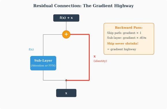
A Concrete Analogy
Think of a company with 30 management layers between the CEO and the front-line workers. Without residual connections, information from the front line has to pass through every layer of management to reach the CEO. At each level, managers summarize, filter, and inevitably distort the message. By the time it reaches the top, the original information is barely recognizable. And when the CEO sends feedback down, the same 30-layer game of telephone distorts it beyond usefulness.
Residual connections are like giving every employee a direct email line to every other employee. The management layers still exist — they still do their processing, their summarizing, their value-added transformations. But the raw information also flows directly through, bypassing the chain entirely. A manager’s job is no longer to replace the information with a fully processed version; it’s to add their insights on top of the original. The original always survives.
“Learning the Residual”
There’s also a conceptual benefit beyond gradient flow. Without residual connections, each block must learn the complete transformation from input to desired output. With residual connections, each block only has to learn the difference between what the input already is and what it should be after this block’s processing:
This “difference” is typically a small, targeted modification — a subtle contextual update from attention, a small knowledge retrieval from the FFN. Learning a small modification to an already-good representation is much easier than learning the entire representation from scratch at every layer.
This also explains an empirical observation: in trained Transformers, the outputs of each block’s attention and FFN sub-layers tend to have much smaller magnitude than the residual stream they’re added to. The sub-layers make small, surgical updates. The residual stream carries the bulk of the information.
Residual Connections in a Transformer Block
In a pre-norm Transformer block, residual connections appear twice — once around the attention sub-layer and once around the FFN:
In the first line, X (the block’s input) is added directly to the attention output. The attention mechanism gets to make its contribution, but it can never erase what was already in X — it can only add to it.
In the second line, X’ (the post-attention representation) is added directly to the FFN output. Same principle: the FFN adds its processing, but the post-attention information always survives.
This means the residual stream — the main flow of information through the network — is never overwritten, only enriched. Each block deposits its contribution into the stream, like tributaries feeding into a river. The river (the residual stream) accumulates information from every block it has passed through.
Residual Connections in the Backward Pass
We already saw this in the worked example, but let’s make it explicit. At the end of block 2, we had:
When we computed the backward pass, the gradient on this sum split into both paths:
The same gradient goes to both the skip path and the FFN path. The skip path gives X^(2)_mid its gradient immediately — no matrix multiplication, no activation function derivative, no potential for shrinkage. The FFN path also contributes a gradient, but it passes through W₂, ReLU, W₁, and LayerNorm, so it’s modified (and potentially shrunk). The total gradient on X^(2)_mid is the sum of both paths — the clean skip gradient plus the FFN-processed gradient.
This splitting happens at every residual connection. In a 2-block model like our example, the gradient from the loss reaches the embeddings via 2^4 = 16 different paths (two residual splits per block, two blocks, and we count each combination). In a 32-block model, there are 2^64 paths. The gradient doesn’t need all of them — it only needs the direct highway (picking the skip at every split) to ensure the signal reaches the earliest layers. All the other paths add information about how the intermediate transformations should change, but even if they all vanished, the highway alone would keep the network trainable.
Layer normalization stabilizes the values flowing through the network by normalizing them to have zero mean and unit variance:
Where μ and σ are the mean and standard deviation computed across the dimensions of x (not across the batch), and γ and β are learned scale and shift parameters. The small ε prevents division by zero.
What Do γ and β Do, and What Is “Identity Initialization”?
The normalization step — subtracting the mean and dividing by the standard deviation — forces every vector to have zero mean and unit variance. But this might be too aggressive. Maybe the network actually needs some dimensions to have larger magnitudes than others, or maybe a slightly non-zero mean is useful for a particular layer’s computations. If we locked the output to exactly zero mean and unit variance, we’d be constraining the network’s expressiveness.
γ (gain) and β (shift) are learnable per-dimension parameters that give the network the freedom to undo the normalization if that turns out to be beneficial. After normalizing to zero mean and unit variance, the network can learn to scale each dimension by γ_i and shift it by β_i:
If the network learns γ = [1, 1, 1, 1] and β = [0, 0, 0, 0], the output is exactly the normalized values — the normalization is fully applied. If it learns γ_i and β_i that exactly reverse the normalization, the output equals the original input — as if LayerNorm weren’t there. In between, the network can learn any combination of “how much to normalize” per dimension.
Identity initialization simply means starting γ = [1, 1, ..., 1] and β = [0, 0, ..., 0], which makes the initial behavior “apply normalization fully.” This is a sensible starting point: normalize everything at the start, and let the network learn to relax this during training if it finds that helpful. It’s called “identity” because with these values, the γ · x̂ + β step is the identity function on the already-normalized values — it passes them through unchanged.
In our worked example, we use γ = [1,1,1,1] and β = [0,0,0,0] throughout, so the scale-and-shift step has no effect, and the LayerNorm output is just the normalized values. But in a real trained model, γ and β would have drifted from their initial values to whatever the loss found useful.
Why Is LayerNorm Needed?
Without normalization, the values in the network can drift to very large or very small magnitudes as they pass through many layers, making optimization unstable. But “making optimization unstable” is vague — let’s be specific about what goes wrong.
In a deep network, each layer’s output is the input to the next layer. If a layer happens to produce values that are much larger than expected — say, vectors with magnitudes of 50 instead of 1 — the next layer’s matrix multiplications will produce even larger values. These large values then enter softmax (in attention) or activation functions, pushing them into regions where gradients are either vanishingly small (saturated softmax, where one position gets 99.99% of the attention) or numerically unstable (exploding values that overflow floating-point precision). Training becomes erratic: some gradient updates are near-zero, others are huge, and the optimizer struggles to make consistent progress.
LayerNorm prevents this by forcing every vector to have a controlled scale before it enters the next computation. It’s like recalibrating a measuring instrument after each measurement — no matter what the previous step produced, the next step always receives inputs in a well-behaved numerical range.
Why Is LayerNorm Applied Multiple Times Per Block?
In a pre-norm Transformer, LayerNorm appears twice per block: once before attention, and once before the FFN. This means a 32-block Transformer has 64 LayerNorms (plus one final LN before the output head — 65 total).
This isn’t redundant. Each sub-layer (attention and FFN) can produce outputs with very different scales. The attention output is a weighted average of value vectors (which can have unpredictable magnitude), and the FFN output passes through a nonlinear activation that can produce extreme values for some inputs. After each of these operations and its residual addition, the vector’s statistics have shifted — its mean and variance may have drifted from the well-behaved range. So we normalize again before the next computation.
Think of it this way: every time the representation passes through a learned transformation (attention or FFN), its numerical properties can drift. Every LayerNorm is a “checkpoint” that resets the scale to something manageable before the next transformation. Without these periodic resets, the drift would compound across blocks. By block 30 or 80, the values could be in a completely uncontrolled range, making training impossible.
There’s also a subtlety about where the LN sits. The residual connection adds the sub-layer’s output to the original input: x’ = x + SubLayer(LN(x)). Because the residual path carries the un-normalized x directly, and each block adds a new contribution to it, the residual stream can grow in magnitude over many blocks. The LayerNorm before each sub-layer ensures that what the sub-layer sees as input is always well-scaled, even if the residual stream itself has drifted. This is one of the key reasons pre-norm (normalize before the sub-layer) works better than post-norm (normalize after the residual add): in pre-norm, the sub-layer always gets a clean, normalized input, and the residual stream remains free to accumulate information without being forced through normalization.
The original Transformer paper applied normalization after each sub-layer (post-norm):
Most modern LLMs use pre-norm instead, applying normalization before each sub-layer:
Pre-norm tends to make training more stable, especially for very deep models, because the residual path remains “clean” — the unnormalized x flows directly through the skip connection without being modified by normalization.
RMSNorm: A Modern Simplification
While LayerNorm is what the original Transformer paper used, most modern LLMs — including LLaMA, Mistral, and their derivatives — have switched to a simplified variant called RMSNorm (Root Mean Square Layer Normalization), introduced by Zhang and Sennrich in 2019.
LayerNorm does two things: it subtracts the mean (centering the values around zero) and divides by the standard deviation (scaling them to unit variance). RMSNorm drops the mean-centering entirely and only rescales by the root mean square of the values:
Notice what’s missing compared to LayerNorm: there’s no mean subtraction, and there’s no β shift parameter. Just a division by RMS and a learnable scale γ.
The key insight from the RMSNorm paper was that most of LayerNorm’s benefit comes from the rescaling (controlling magnitude), not from the recentering (shifting the mean to zero). Removing the mean computation saves about 10-15% of the normalization cost per layer. That might sound modest, but in a 80-block model with two normalizations per block plus one at the output — 161 normalizations per forward pass — the savings compound. And since normalization is applied at every step, to every position, on every training example, even a small per-operation saving translates to real efficiency at scale.
Functionally, RMSNorm and LayerNorm behave very similarly: both keep values in a well-behaved numerical range, both prevent drift across deep layers, and both are applied in the same positions (pre-attention and pre-FFN in pre-norm architectures). The difference is purely in which statistics are computed. For the conceptual understanding we’re building, everything we said about why normalization is needed, why it appears multiple times per block, and why pre-norm beats post-norm applies equally to RMSNorm. It’s a drop-in replacement that trades a tiny amount of theoretical flexibility for a meaningful efficiency gain.
A Complete Transformer Block
Let’s now assemble these components into a single Transformer block. In a decoder-only model (GPT-style), one block looks like this:
Layer Norm on the input
Masked Multi-Head Self-Attention (causal, so no peeking at future tokens)
Add the residual (input + attention output)
Layer Norm on the result
Feedforward Network (expand, GELU, contract)
Add the residual (step 3 output + FFN output)
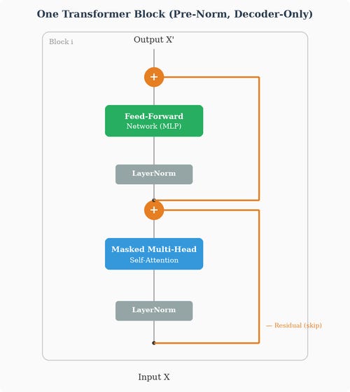
Formally, for a block with input X:
That’s it. That’s the entire block. And a full Transformer is just this block repeated N times, one after another, with each block having its own independent set of learned weights (W_Q, W_K, W_V, W_O for attention; W₁, W₂ for the FFN; γ, β for each LayerNorm).
GPT-2 Small uses 12 blocks (larger GPT-2 variants go up to 48). GPT-3 uses 96. LLaMA 7B uses 32. LLaMA 70B uses 80. Each block refines the representation, building increasingly abstract and contextual understanding. The first few layers tend to handle syntax and local patterns. The middle layers capture semantic relationships and factual knowledge. The final layers prepare the representation for the specific prediction the model needs to make.
Stacking N Blocks: Depth of Processing
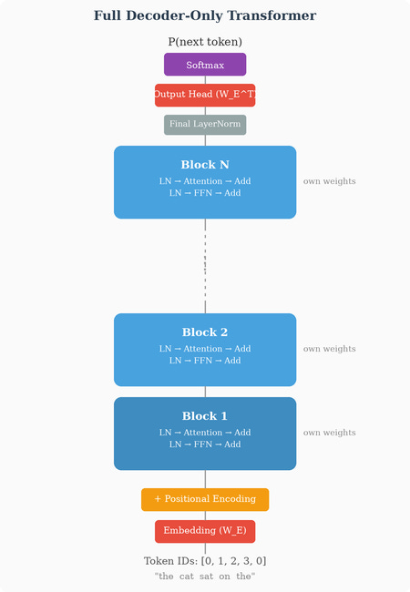
When we say a Transformer has “N layers” or “N blocks” — GPT-2 has 12, GPT-3 has 96, LLaMA 7B has 32 — we mean that the attention-plus-FFN pattern is repeated N times sequentially in depth. The output of block 1 becomes the input of block 2. The output of block 2 becomes the input of block 3. And so on, up to block N. It’s exactly like the forward pass through hidden layers in Part 1’s MLP: data flows through one transformation after another, in order.
Crucially, each block has its own independent set of weights. Block 1 has its own W_Q^(1), W_K^(1), W_V^(1), W_O^(1), W_1^(1), W_2^(1), and LayerNorm parameters. Block 2 has a completely separate set — W_Q^(2), W_K^(2), W_V^(2), and so on. No weights are shared across blocks. Each block is a fresh set of learnable parameters. When we say a 7-billion-parameter model, most of those billions are simply the sum of the weights of every block stacked in the model, plus the embeddings.
Information flows through this stack in a single forward pass, always in the same direction: embeddings (plus positional info) → block 1 → block 2 → ... → block N → output head → softmax. Within each block, all positions of the sequence are processed in parallel — this is where the Transformer’s famous parallelism lives. The attention operation looks at every position simultaneously. But across blocks, there is strict sequential dependency: block 3 can’t start until block 2 has finished producing its output.
A useful mental model: each block is one round of “reading and thinking” about the sequence.
Block 1 sees the raw embeddings (the superposition of all senses we discussed earlier) and produces an initial round of contextualization — mostly local syntax, morphological patterns, surface-level relationships.
Block 2 operates on block 1’s output. Its inputs are no longer raw embeddings but already-contextualized vectors. So block 2 can build on that first round, picking up slightly more abstract patterns — short-range dependencies, simple phrase structure.
By block 20 or 50 or 80, the vectors at each position have been enriched many times over. Each round of attention has pulled in additional information from across the sequence. Each FFN has added more processing per position. The representations have become deeply contextualized and highly abstract.
Empirical studies of trained Transformers — via probing experiments, attention visualization, and mechanistic interpretability research — broadly support this picture: early blocks handle surface features and local patterns, middle blocks capture semantic composition and factual associations, and later blocks refine the representation for the specific output task. In an LLM, the final block’s output at the final position is what passes through the output head to generate the next token.
Depth matters because each block can only do a limited amount of work. A single block can mix information across positions once through attention, and apply one FFN transformation per position. To build up deep reasoning — tracking long chains of dependencies, performing implicit multi-step inference, integrating many pieces of evidence — you need many rounds of this. Depth gives the model the computational budget for genuinely complex thinking. This is why the most capable LLMs tend to be very deep (80 or more blocks) as well as wide (large d_model).
Sensible Values: Real-World Configurations
To anchor all this with concrete numbers, here are the configurations of some well-known models:
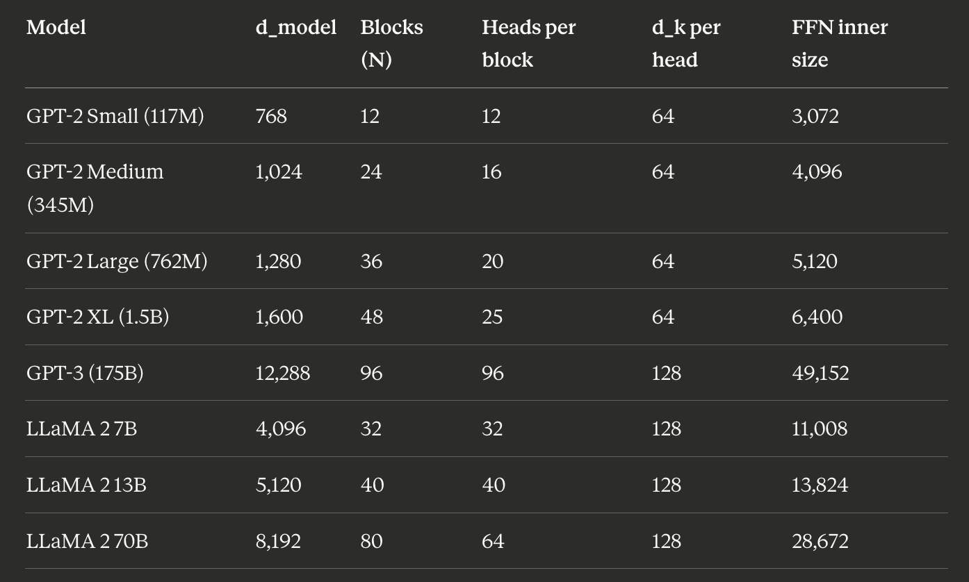
A few patterns worth noticing:
d_k per head stays fairly constant across model sizes — almost always 64 or 128. What changes as models grow is how many heads fit into d_model. This is a deliberate design choice: each head needs enough dimensions to form meaningful Q/K dot products, and below about 64 dimensions the attention signal gets noisy.
FFN inner dimension is about 4× d_model. This ratio has stayed remarkably consistent across almost all Transformer models. The FFN expands the representation to a 4×-wider space for non-linear processing, then contracts back.
Depth and width scale together as models grow, but not at the same rate. Going from GPT-2 Small (117M) to GPT-3 (175B) — a 1500× increase in parameters — d_model grows 16× while the number of blocks grows 8×. The parameter count is dominated by the N × d_model^2 product, which grows about 2000×.
Total parameters are dominated by the block weights. Each block contributes roughly 12 × d_model^2 parameters (4× from the Q/K/V/O attention matrices, and 8× from the two FFN matrices, since one is d_model × 4d_model and the other is 4d_model × d_model). Multiply by N blocks and you have the bulk of the model’s parameters.
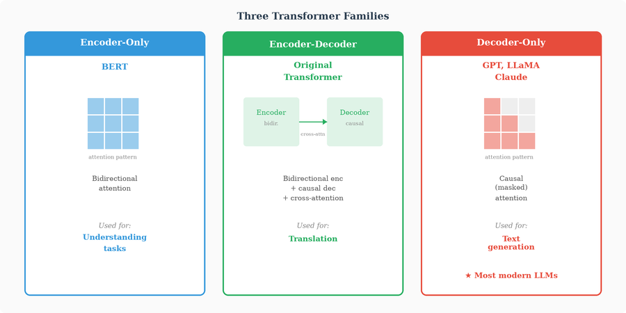
There's no universal law dictating these exact ratios — they emerged from years of empirical experimentation. The Kaplan et al. (2020) and Hoffmann et al. (2022, the "Chinchilla" paper) scaling laws explored how these hyperparameters should scale together for optimal performance at a given compute budget, and modern models are configured following those findings. But fundamentally, every extra block adds another round of attention and FFN processing, every extra head adds another way to attend in parallel within a block, and the choice of how to allocate compute between depth and width is a design tradeoff.
Grouped Query Attention (GQA)
In the multi-head attention we described, every head has its own W_Q, W_K, and W_V. If a model has 64 heads, that means 64 independent query matrices, 64 independent key matrices, and 64 independent value matrices. This is the standard setup — called Multi-Head Attention (MHA).
But there’s a practical problem that shows up during inference (text generation). When the model generates text token by token, it needs to keep the key and value vectors from all previous tokens in memory — this is the KV-cache (which we’ll cover properly in Part 3). With 64 heads, each storing key and value vectors for every position in the sequence, across every block in the model, the KV-cache grows enormous. For a 70-billion parameter model generating a long document, the KV-cache alone can consume tens of gigabytes of GPU memory.
Grouped Query Attention (GQA), introduced by Ainslie et al. in 2023, addresses this by observing something surprising: the model doesn’t actually need 64 independent sets of keys and values. It still benefits from 64 independent sets of queries (each query head learns a different “question to ask”), but the keys and values can be shared across groups of query heads without significantly hurting quality.
Here’s how it works mechanically. Instead of 64 query heads and 64 KV heads, GQA might use 64 query heads but only 8 KV heads. The 64 query heads are divided into 8 groups of 8. All 8 query heads in a group share the same key and value projections:
Group 1: query heads 1–8 all use W_K^1 and W_V^1
Group 2: query heads 9–16 all use W_K^2 and W_V^2
...
Group 8: query heads 57–64 all use W_K^8 and W_V^8
Each query head still has its own W_Q — so each head still asks its own question. But when computing K and V, eight different query heads look at the same keys and values. The attention scores and outputs are still computed per query head (since Q differs), so each head can still produce a different attention pattern. They just do it from a shared set of keys and values.
This sits on a spectrum between two extremes:
Multi-Head Attention (MHA): every head has its own Q, K, V. Maximum expressiveness, maximum KV-cache size. This is what the original Transformer paper proposed.
Multi-Query Attention (MQA): every head has its own Q, but all heads share a single K and single V. Minimum KV-cache size, but some quality degradation. This was proposed by Shazeer in 2019.
Grouped Query Attention (GQA): a middle ground. Heads are grouped, and each group shares K/V. You choose how many KV heads to use — anywhere between 1 (MQA) and H (MHA).
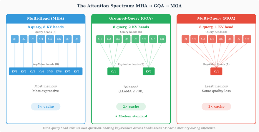
Why does sharing keys and values work? The intuition is that the “what do I contain?” (key) and “what do I give?” (value) roles are less diverse across heads than the “what am I looking for?” (query) role. Many heads ask different questions about the same input, but the input is the same — the key and value representations don’t need as much per-head specialization. Different query heads can extract different information from the same key-value pairs simply by asking different questions.
The practical impact is significant. LLaMA 2 70B uses 64 query heads but only 8 KV heads (8 groups of 8). This reduces the KV-cache memory by 8× compared to standard MHA — from “barely fits on a high-end GPU” to “comfortably fits.” The quality loss is negligible in practice, and in some benchmarks GQA models actually perform slightly better than MHA models, likely because the shared keys and values act as a mild form of regularization.
GQA has become the standard for large models. LLaMA 2 (70B), LLaMA 3, Mistral, and most recent open-source architectures use it. For smaller models where the KV-cache isn’t a bottleneck, standard MHA is still common. The choice depends on the inference constraints you’re designing for.
The Output Head
After passing through all N Transformer blocks, the model has a sequence of vectors — one per input token — each of dimension d_model. For next-token prediction, we only care about the last position (or, during training, every position, since we predict the next token at every position simultaneously).
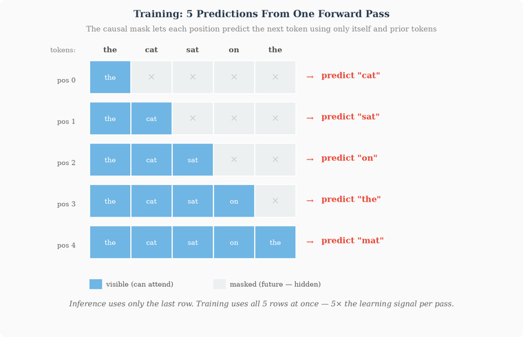
This gives us five training signals from one forward pass. The five per-position cross-entropy losses are averaged into a single scalar, and then a single backward pass propagates all five error signals at once. This works because the gradient of an average of losses is just the average of the individual gradients: where the five error signals reach a shared weight (and nearly every weight is shared across positions), their contributions simply add up. So one traversal of the network accumulates all five corrections — you do not run backpropagation five separate times. Without this trick, training would be 5× slower: you'd need a separate forward and backward pass for each prefix length.
The output vector passes through a final linear layer that projects from d_model to the full vocabulary size:
Where W_head has shape (d_model × V), with V being the vocabulary size. The result is a vector of V logits — the raw, unnormalized scores we introduced earlier — one per token in the vocabulary.
Many models use weight tying: the output projection matrix W_head is set to be the transpose of the embedding matrix W_E. This makes intuitive sense — the embedding matrix maps from vocabulary space to model space, and the output projection maps from model space back to vocabulary space. They’re doing inverse operations, so sharing the weights (a) reduces the total parameter count and (b) creates a geometric consistency where producing a token is literally “finding the token whose embedding is most similar to the output vector.”
The logits are then passed through a softmax function to produce a probability distribution:
This gives the model's predicted probability for every token in the vocabulary being the next token. During training, this distribution is compared against the actual next token using cross-entropy loss (generalizing the binary cross-entropy we saw in Part 1 to a multi-class setting):
Since the true next token is a one-hot vector (all zeros except for the correct token), this simplifies to:
Which is just the negative log probability the model assigned to the correct next token. If the model was confident and correct (high hat{p}_correct), the loss is small. If the model was confident and wrong, the loss is enormous. Same principle as the binary case in Part 1, extended to 50,000+ classes.
Generating Text: Sampling Strategies
During inference (text generation), the model produces a probability distribution over the vocabulary and must select a single token. The simplest approach is greedy decoding: always pick the token with the highest probability. But this often produces repetitive, generic text.
More sophisticated strategies include:
Temperature: before softmax, divide the logits by a temperature parameter T:
T = 1: standard probabilities
T < 1: distribution becomes sharper (more confident, more deterministic)
T > 1: distribution becomes flatter (more random, more creative)
Top-k sampling: sort tokens by probability, keep only the top k tokens, redistribute their probabilities, and sample from this truncated distribution.
Top-p (nucleus) sampling: instead of a fixed k, keep the smallest set of tokens whose cumulative probability exceeds p (e.g., 0.9). This adapts to the model’s confidence — sometimes only 5 tokens might cover 90% of the probability mass, other times it might be 500.
In practice, most systems combine temperature with top-p sampling for a good balance of coherence and variety.
The Complete Picture: From Text In to Prediction Out
We’ve now covered every component of the Transformer individually. Before we move to the worked example, let’s step back and see the full architecture as a single, coherent pipeline. This is the view you should hold in your head — the complete journey that a piece of text takes from raw characters to a probability distribution over the next token.
Step 1: Tokenization. Raw text enters the system as a string of characters. The tokenizer (BPE, SentencePiece, or similar) breaks it into a sequence of integer token IDs. “The cat sat on the” might become [1, 4523, 8891, 312, 1]. This step is purely mechanical — no neural network is involved. The tokenizer is a fixed algorithm, trained once on a large text corpus, then frozen. Its job is to convert the infinite variety of text into a finite vocabulary of integer IDs that the model can work with.
Step 2: Embedding lookup. Each token ID is used to index into the embedding matrix W_E, pulling out a dense vector of d_model dimensions. Token ID 4523 retrieves row 4523 of W_E. The sequence of integers becomes a sequence of vectors — a matrix of shape (sequence_length, d_model). This is where discrete symbols cross the bridge into continuous space.
Step 3: Positional encoding. Position information is injected, either by adding sinusoidal vectors, adding learned positional embeddings, or (in models using RoPE) by rotating the vectors inside the attention computation. After this step, two instances of the same token at different positions have different vector representations, so the model can distinguish word order.
Step 4: The Transformer blocks. This is the core of the model, where all the “thinking” happens. The sequence of vectors passes through N blocks stacked in series — block 1’s output feeds into block 2, block 2’s output feeds into block 3, and so on up to block N. Each block performs the same two-step pattern:
Attention sub-layer: every position looks at every previous position (via causal masking), computes relevance scores through the Q/K/V mechanism across multiple heads, gathers information from relevant positions, and combines it through the output projection W_O. This is the “communication” step — positions exchange information.
FFN sub-layer: each position independently passes through a small MLP (the gate/up/down projections in modern models, or the simpler W₁/W₂ in the original). This is the “thinking” step — each position processes the information it gathered.
Both sub-layers are wrapped in LayerNorm (or RMSNorm) and residual connections, ensuring stable training and clean gradient flow. Each block has its own independent weights — no sharing between blocks.
After N blocks, the representation at each position has been enriched by N rounds of attention and N rounds of per-position processing. Early blocks tend to capture surface-level patterns (syntax, local context), middle blocks capture semantic relationships and factual knowledge, and later blocks refine the representation toward the specific prediction the model needs to make.
Step 5: Final normalization. One last LayerNorm (or RMSNorm) is applied to the output of the final block, ensuring the values are in a well-behaved numerical range before the output computation.
Step 6: Output head. The vector at the last position — the position that’s predicting what comes next — is projected from d_model dimensions to vocabulary-size dimensions through the output head matrix. With weight tying, this is just the transpose of the embedding matrix: the dot product of the final vector with each token’s embedding row produces one logit per token. Tokens whose embeddings are most aligned with the final hidden vector get the highest logits.
Step 7: Softmax. The logits are converted to a probability distribution via softmax. Every token in the vocabulary now has a probability between 0 and 1, and all probabilities sum to 1. The model has answered the question: “Given everything I’ve seen so far, how likely is each possible next token?”
Step 8: Sampling or loss. During inference (text generation), a token is sampled from this distribution using temperature, top-k, or top-p strategies, and the process repeats from step 1 with the new token appended. During training, the probability assigned to the actual next token is compared against 1.0 via cross-entropy loss, producing the scalar error signal that drives backpropagation through every parameter in the pipeline.
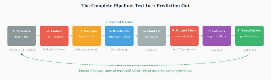
That’s the entire architecture. Eight steps, in order, every time. The model sees text, converts it to vectors, processes those vectors through many rounds of attention and feedforward computation, and produces a probability distribution over what comes next. Everything we covered in the preceding sections — embeddings, positional encoding, Q/K/V projections, multi-head attention, causal masking, the FFN and its variants, residual connections, LayerNorm — slots into this pipeline at a specific, well-defined point. There are no hidden steps, no additional mechanisms we haven’t discussed.
Now let’s see it in action with real numbers.
IV. An End-to-End Worked Example
Now let’s see the whole thing in action — one complete forward pass through all eight steps, then one complete backward pass, with every number computed explicitly. Just like Part 1, we’ll follow every calculation so that nothing is left as a black box.
To make this tractable by hand, we’ll use a deliberately tiny model. Real LLMs have billions of parameters and thousands of dimensions; ours will have dozens of parameters and single-digit dimensions. But the mechanics are identical — what changes with scale is the size of the matrices, not the operations themselves.
Setup
Our tiny Transformer will have:
Vocabulary size V = 8
Model dimension d_model = 4
Number of heads per block H = 2, so d_k = d_v = d_model/H = 2
Number of blocks N = 2
FFN inner dimension d_ff = 8 (2× d_model; real models use 4×, but we’ll keep it small)
Activation in the FFN: ReLU (matching Part 1 for continuity)
Weight tying: the output projection W_head equals W_E^T (so the embedding matrix is used at both input and output)
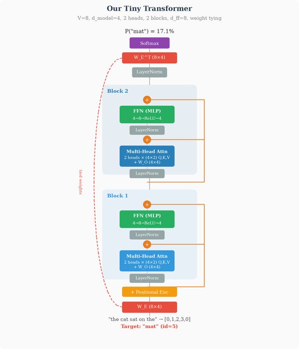
Our vocabulary:
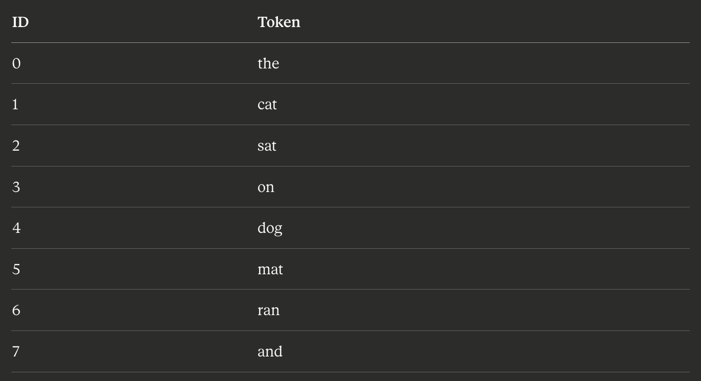
Input sentence: “the cat sat on the” → token IDs [0, 1, 2, 3, 0] Target next token: “mat” → token ID 5
We want the model to learn that after “the cat sat on the,” the likely next word is “mat.” Of course, with random weights it won’t predict this well at first. What we’ll see is exactly one forward pass (to make a prediction and compute loss), then one backward pass (to compute gradients), then one weight update.
Step 1: From Tokens to Vectors
The first step is to convert each token ID into a vector via the embedding matrix W_E (shape V × d_model = 8 × 4). Its initial values (chosen deliberately simple for this example):
Row 0 is the vector for “the,” row 5 is the vector for “mat,” and so on.
For our input sequence [0, 1, 2, 3, 0], we look up rows 0, 1, 2, 3, and 0 again:
Five rows for five positions. Notice that positions 0 and 4 are identical — both are the vector for “the.” Without positional information, the model would see these two positions as indistinguishable, and the whole sequence would be order-invariant.
To fix this, we add a positional encoding W_P (chosen simply, purely for this example):
Adding E + W_P gives us X^(0), the input to the first Transformer block:
Step 2: Layer Normalization (Pre-Attention)
Inside block 1, the first operation is a LayerNorm applied to X^(0). LayerNorm normalizes each row independently, computing the mean and standard deviation across the 4 dimensions of that row, then rescaling.
For row 0 of X^(0) (the vector [0.10, 0.20, 0.00, 0.10]):
Mean: μ = (0.10 + 0.20 + 0.00 + 0.10)/4 = 0.10
Variance: σ^2 = [(0)^2 + (0.10)^2 + (-0.10)^2 + (0)^2]/4 = 0.005
Standard deviation: σ = √{0.005 + ε} ≈ 0.0708 (using ε = 10^-5)
Normalized: (x - μ)/σ = [0, 0.10, -0.10, 0]/0.0708 = [0, 1.413, -1.413, 0]
Then scaled and shifted: γ ⊙ x̂ + β. With γ = [1,1,1,1] and β = [0,0,0,0] (the identity initialization we’re using throughout), the output is just [0, 1.413, -1.413, 0].
You might wonder what this scale-and-shift step is doing, given that with these values it has no visible effect. We covered γ and β in detail in the architecture section, but it’s worth reinforcing here in the context of actual numbers.
The normalization step forcefully rescaled this vector to have zero mean and unit variance. But maybe the attention mechanism that comes next would work better if certain dimensions had slightly different magnitudes — perhaps dimension 2 should be amplified, or the whole vector needs a small positive shift. γ and β are learnable parameters (just like weights and biases) that let the network undo, modify, or preserve the normalization as it sees fit. With γ = [1,1,1,1] and β = [0,0,0,0], we’re at the identity initialization: the network starts by fully applying the normalization, and during training, γ and β will drift to whatever values the loss function finds useful. In a trained model these values are typically close to but not exactly at their initial values — the network has learned a slight per-dimension rescaling that helps downstream computations.
In our worked example, since we’re showing one forward and backward pass before any training has happened, γ and β are still at their initial values and the scale-and-shift is a no-op. But they’re there, they’re learnable, and they receive gradients just like every other parameter in the network.
Applying the same to all five rows:
This is what feeds into the multi-head attention.
Step 3: Multi-Head Self-Attention — First Head
Before we proceed with calculations, let’s settle a question that’s been hanging in the air: is a single head the same as “self-attention”?
Yes. Self-attention is defined by where the queries, keys, and values come from: in self-attention, all three are computed from the same sequence. (In cross-attention, used in the original Transformer’s decoder, queries come from the decoder and keys/values come from the encoder — the decoder attends to the encoder’s output.) Self-attention is the mechanism we’ve been describing all along, and it doesn’t say anything about how many heads are involved. A single-head self-attention is already self-attention — it’s just self-attention with H = 1 parallel computation. The Q/K/V mechanism with one head IS self-attention.
Multi-head self-attention means running several self-attention computations in parallel — each with its own W_Q, W_K, W_V matrices — and combining their outputs. Each individual head is a full self-attention operation in its own right, just working in a lower-dimensional subspace. Let’s see this concretely by computing head 1 in detail first, then head 2, then seeing how they combine.
Head 1: Computing Q, K, V
Head 1 has its own three weight matrices (shape d_model × d_k = 4 × 2). Initial values:
(Superscript (1,1) means “block 1, head 1.”)
We multiply the normalized input X^(0)_LN by each of these to get Q, K, V for head 1:
Each row is the query vector for one position — a 2-dimensional vector (because d_k = 2). Position 0’s query is [-0.141, 0.141], position 1’s is [0.734, -0.192], and so on.
Let me show the first-row computation explicitly so the matrix multiplication is fully transparent. For position 0: query = [0.000, 1.413, -1.413, 0.000] · W_Q^(1,1) gives two numbers:
First component: 0.000 · 0.5 + 1.413 · 0.1 + (-1.413) · 0.2 + 0.000 · 0.0 = 0.141 - 0.283 = -0.141 ✓
Second component: 0.000 · 0.1 + 1.413 · 0.4 + (-1.413) · 0.3 + 0.000 · 0.2 = 0.565 - 0.424 = 0.141 ✓
Similarly:
So every position now has its own query vector, its own key vector, and its own value vector — all in a 2-dimensional subspace specific to head 1.
Head 1: Attention Scores
Attention scores come from Q K^T / √{d_k}. With d_k = 2, we divide by √{2} ≈ 1.414.
The dot product between position 4’s query and position 0’s key:
Doing this for every pair (i, j) gives the full score matrix:
Each row is how much a query at that position “liked” each key. Row 4, for example, shows how the query for the last “the” scored against every key from position 0 to 4. All numbers are small, reflecting the fact that this model has random weights — there are no strong preferences yet.
Head 1: Causal Mask and Softmax
Because we’re building a decoder-only (autoregressive) model, each position must only attend to previous positions (and itself). We apply a causal mask — adding -∞ to all upper-triangular entries:
Now we apply softmax row by row. For row 1, [0.035, 0.114, -∞, -∞, -∞]:
(The -∞ entries softmax to 0.) So position 1’s query attends 48% to position 0 and 52% to position 1 (itself).
Doing this for all rows:
This is the attention matrix for head 1. Row 4 tells us that the last "the" is attending roughly uniformly to all five positions (about 20% each). That's expected — with random weights, nothing has been learned to make the model prefer any particular past position. After training, we'd see much spikier distributions.
Head 1: Output
The output of head 1 is A^(1,1) V^(1,1). For the last row (position 4):
out4(1,1)= 0.201⋅[−0.706,0.424]+0.201⋅[0.227,−0.192]+0.196⋅[−0.680,0.417]+0.199⋅[0.440,−0.314]+0.204⋅[−0.523,0.284]
Computing each term and summing:
For all positions:
This is a (5, 2) matrix: five positions, each now represented in head 1’s 2-dimensional output space. That’s all head 1 does. It’s a complete self-attention computation in a 2-dimensional subspace.
Step 4: Multi-Head Self-Attention — Second Head (in Parallel)
Here’s where the “multi-head” part matters. Head 2 does exactly the same kind of computation as head 1, but with its own independent weight matrices:
Note: these are different matrices from head 1’s. That’s the whole point. Both heads see the same input X^(0)_LN, but they project it into different subspaces. Because the projections are different, the queries, keys, and values are different, and therefore the resulting attention patterns and outputs are different. This gives the model two independent “perspectives” on the same sequence at the same depth.
Running the same calculation pipeline — Q^(1,2) = X^(0)_LN W_Q^(1,2), and so on — head 2 produces its own attention weights and output:
Compare this to head 1’s attention matrix. Row 1 here is [0.413, 0.587]; in head 1 it was [0.480, 0.520]. Different weights, different patterns. With only random initialization the differences are modest, but after training, different heads typically learn to focus on very different things — one head might track syntactic agreement, another might resolve coreferences, another might focus on nearby tokens, and so on. The capacity for diversity comes from having separate W_Q, W_K, W_V per head.
Head 2’s output:
About “Running in Parallel”
Note the word parallel. Both heads operate on the same input X^(0)_LN. Neither depends on the other’s output. On a GPU, you’d compute head 1 and head 2 simultaneously on different cores. They’re independent computations that share the same input — that’s all “parallel” means here.
And critically: they are not averaged. This is a common misconception. Many people assume multi-head attention combines the heads by averaging their outputs. It doesn’t. The heads are concatenated.
Step 5: Concatenation and Output Projection
Head 1 output is shape (5, 2). Head 2 output is shape (5, 2). To combine them, we concatenate along the last dimension, giving a matrix of shape (5, 4):
Look at the structure: the first 2 columns are head 1’s output, the last 2 columns are head 2’s output. They sit side by side. Each row now has 4 numbers — the first 2 from head 1, the second 2 from head 2.
Why concatenate instead of averaging? Because the heads operate in different subspaces. Averaging would force their outputs to live in the same 2D space, which would defeat the purpose of having multiple heads. Concatenation keeps each head’s contribution distinct.
Now comes the key combining step: a learned output projection W_O^(1) of shape (d_model, d_model) = (4, 4):
The matrix multiplication concat^(1) · W_O^(1) mixes all 4 concatenated values of each row (2 from each head) into a new 4-dimensional representation:
This is the final output of the multi-head attention sub-layer. W_O^(1) is also a learnable parameter — it learns how to best combine the heads. In a sense, W_O learns which aspects of which heads to emphasize when producing the final output. The heads produce diverse views; W_O chooses how to fuse them.
Step 6: Residual Connection and FFN
The residual connection adds the attention output back to the original input (the pre-LN input, X^(0), not the post-LN input):
This residual is essential — it means gradients during the backward pass have a direct path from X^(1)_mid back to X^(0), bypassing the attention mechanism entirely. Without this, deep Transformers would be very difficult to train.
Next, another LayerNorm (normalizing X^(1)_mid to zero mean and unit variance at each position), then the feedforward network. This is where the MLP from Part 1 shows up inside the Transformer.
The FFN has two weight matrices and two bias vectors:
W_1^(1) of shape (4, 8): takes the 4-dimensional vector at each position and expands it to 8 dimensions
b_1^(1): bias of length 8
W_2^(1) of shape (8, 4): contracts the 8-dimensional representation back to 4 dimensions
b_2^(1): bias of length 4
This is exactly the structure of Part 1’s MLP: input layer (4 neurons) → hidden layer (8 neurons) → output layer (4 neurons). The hidden layer has twice as many neurons as the input, which is the “expand” step. The output layer contracts back to the original size.
Let's trace position 4 (the last "the") through the FFN step by step.
After LayerNorm 1b, position 4's vector is:
First layer (expand):
This is the same computation we did for every hidden neuron in Part 1: for each of the 8 neurons in the hidden layer, compute the weighted sum of all 4 inputs plus the bias. The result is an 8-dimensional vector:
Each number is one neuron’s pre-activation value. Neuron 1 computed 0.525 (a moderately positive response to this input), neuron 2 computed -0.302 (a negative response), neuron 4 computed 0.467, and so on.
Activation (ReLU):
ReLU zeroes out the negative values. Neurons 2, 5, and 7 (which had values -0.302, -0.435, -0.060) are now dead — they contribute nothing to the output. Only neurons 0, 1, 3, 4, and 6 are “active.” This is the sparse activation pattern: 5 out of 8 neurons fire for this particular input. A different input would activate a different subset.
This is identical to what happened in Part 1 when hidden neuron h3 had a pre-activation of -0.057 and ReLU set it to 0. Same mechanism, just with more neurons.
Second layer (contract):
Only the 5 active neurons contribute to this sum. Each active neuron’s contribution is determined by its activation value multiplied by its column in W₂. The dead neurons multiply by zero and contribute nothing. The result is a 4-dimensional vector — back to d_model — representing the FFN’s processed output for this position.
The full FFN output for all five positions:
Each row was processed independently through the same W_1^(1), ReLU, W_2^(1) — each with different activations, different sets of neurons firing, but the same weights. This is one complete MLP pass, applied identically to each of the five positions.
After the FFN, another residual add:
This is the final output of block 1 — five positions, each enriched with contextual information from attention and further processed by the FFN. X^(1) is what enters block 2.
Step 7: Block 2
Block 2 has the same structure as block 1 — LayerNorm, multi-head attention (same 2 heads), residual, LayerNorm, FFN, residual — but with its own independent set of weights. Everything we did in steps 2 through 6 repeats, but with different numbers.
I won’t walk through all the block 2 calculations step by step (they’re mechanically identical to block 1), but the final output is:
Each row is the representation at that position, now having passed through two complete rounds of attention and FFN processing. Compared to the embeddings we started with, these vectors have been enriched by information from all previous positions (via attention) and further processed by nonlinear transformations (via the FFNs).
Step 8: Final LayerNorm, Output Head, Softmax
After all blocks, a final LayerNorm is applied:
For next-token prediction, we only care about the last position — position 4, whose vector is h = [-0.378, 1.335, -1.377, 0.420]. This is what the model has built up through the entire network as its final understanding of “what should come next after ‘the cat sat on the’”.
Now we convert this 4-dimensional vector into logits over the vocabulary using the output head. With weight tying, W_head = W_E^T, so the logit for each token t is simply h · W_E[t] — the dot product between the final hidden vector and that token’s embedding row.
Computing each:
logit(the) = (-0.378)(0.1) + (1.335)(0.2) + (-1.377)(0.0) + (0.420)(0.1) = -0.038 + 0.267 + 0 + 0.042 = 0.271
logit(cat) = (-0.378)(0.3) + (1.335)(0.1) + (-1.377)(0.2) + (0.420)(0.0) = -0.113 + 0.134 - 0.275 = -0.255
logit(mat) = (-0.378)(0.1) + (1.335)(0.4) + (-1.377)(0.2) + (0.420)(0.3) = -0.038 + 0.534 - 0.275 + 0.126 = 0.347
Full logits:
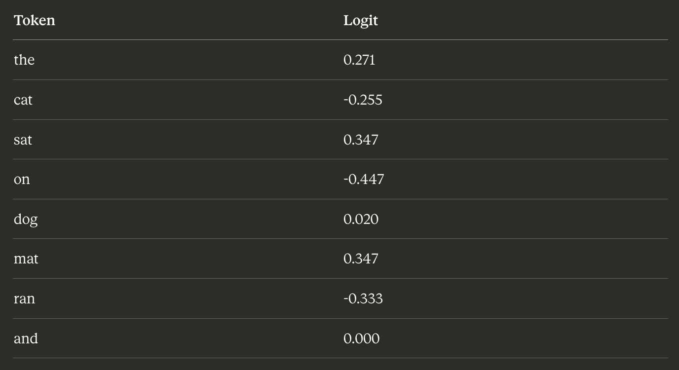
Softmax converts these to probabilities. Let me show the first few calculations:
e^0.271 ≈ 1.311
e^-0.255 ≈ 0.775
e^0.347 ≈ 1.415
e^-0.447 ≈ 0.639
e^0.020 ≈ 1.020
e^0.347 ≈ 1.415
e^-0.333 ≈ 0.717
e^0.000 = 1.000
Sum = 8.292.
Dividing each:
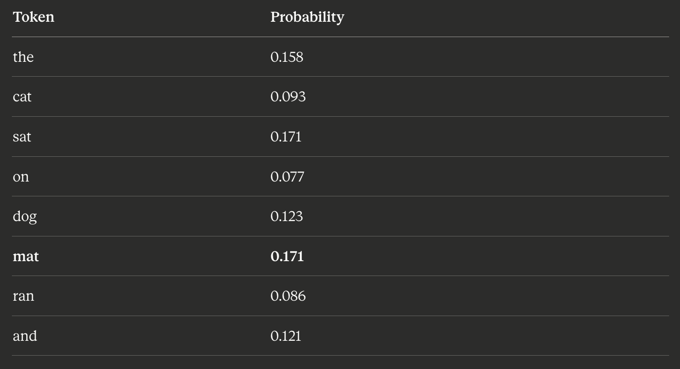
The model assigns probability 0.171 to the correct answer “mat.” That’s barely above uniform (1/8 = 0.125). With random weights, this is about what we’d expect — the model has no reason to prefer “mat” over “sat” (note they’re tied at 0.171), and it gives reasonable probability to everything. Tokens like “on” and “ran” get pushed slightly down.
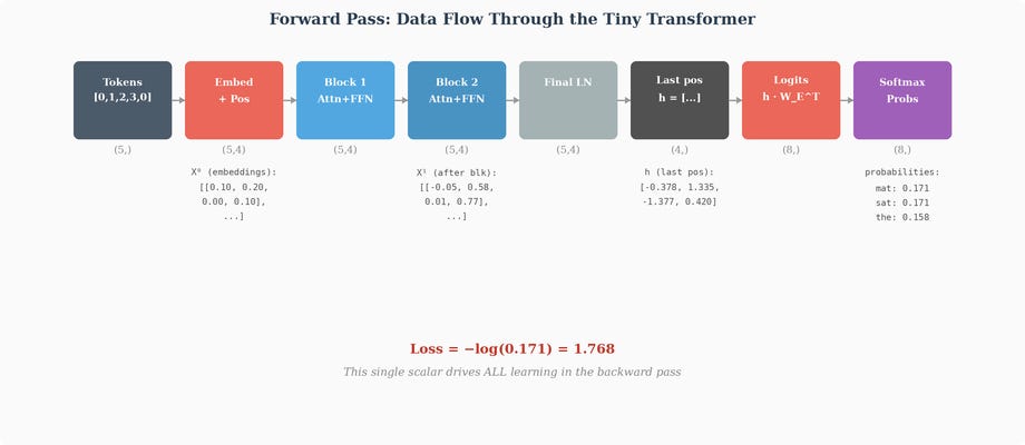
Step 9: The Loss
Cross-entropy loss against the target (token 5, “mat”):
This is our scalar loss value. A loss of 1.768 means the model is “surprised” by the correct answer — specifically, it assigned only 17.1% probability, which is mediocre. Ideally the model would assign near 100% probability to “mat,” giving a loss near 0. For comparison, a uniform model would give -log(1/8) = log(8) ≈ 2.08, so we’re doing slightly better than random — but not much.
One simplification to flag: as we saw in The Output Head, a real training step computes a prediction at every position and averages all of those cross-entropy losses into one scalar. Here we're tracing only the last position's prediction ("the cat sat on the" → "mat") so the arithmetic stays tractable by hand. The mechanics are identical — the only difference is whether the single scalar at the top of the backward pass is one position's loss or the mean of all of them. Everything that follows works the same way regardless.
Step 10: The Backward Pass — Gradient at the Output
Now we trace the chain rule backward through the entire network. The first gradient is the derivative of the loss with respect to the logits. For softmax followed by cross-entropy, there’s a beautifully clean formula:
where p_i is the predicted probability and y_i is 1 if i is the target, else 0. For our prediction:
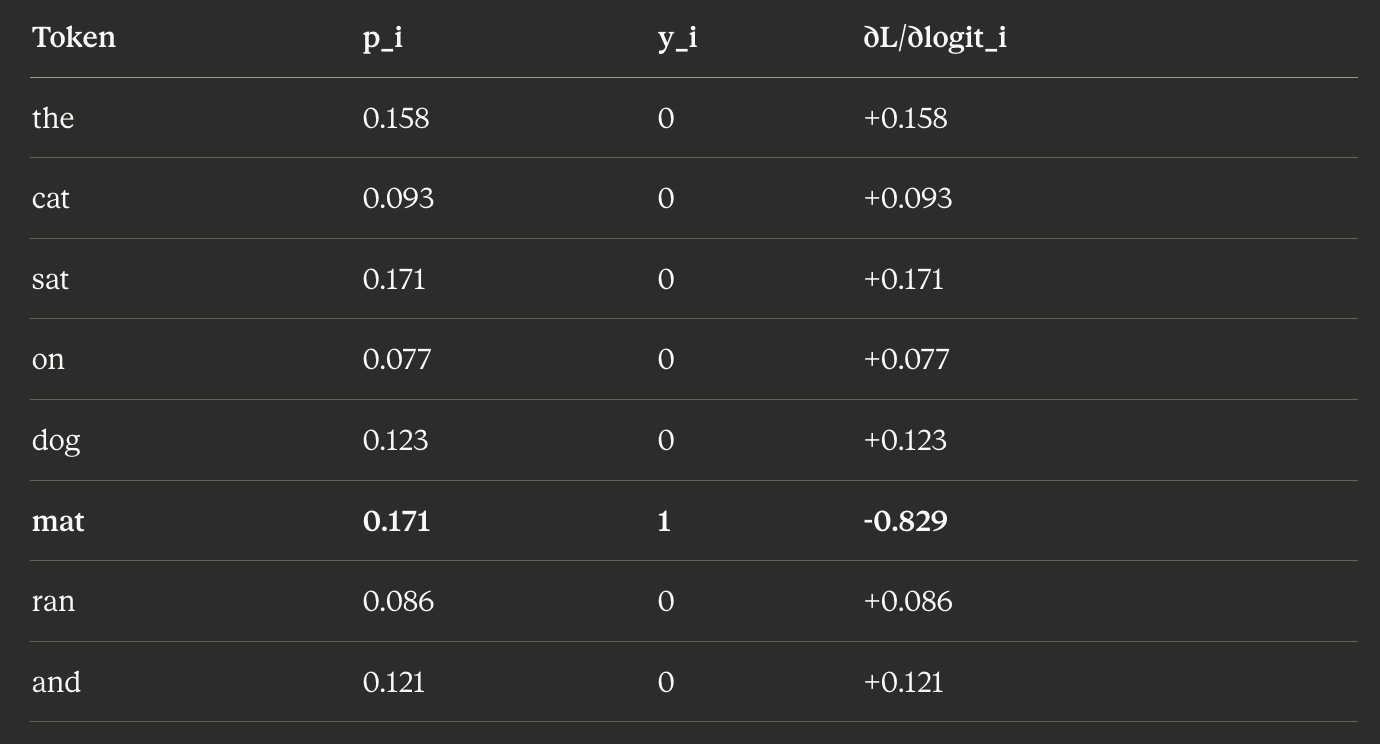
Pause to notice what this says. The gradient is negative for the target (”mat” gets -0.829) and positive for all the other tokens. In gradient descent, we move in the negative gradient direction, so:
The logit for “mat” will go up (we subtract a negative → add)
The logits for all other tokens will go down
Which is exactly what we want: make the correct answer more probable, make the incorrect answers less probable. That single -0.829 on “mat” is the error signal that’s about to ripple backward through every matrix in the network.
Step 11: From Logits Back to the Final Hidden State
The logits were computed as logits = h · W_E^T. Using the matrix calculus rule for this kind of product:
This is a vector-matrix product: an 8-dimensional gradient dotted into the 8×4 matrix W_E, giving a 4-dimensional result. Working through:
This is the gradient telling us how the final hidden vector should change to reduce the loss. It says: decrease component 1 (the second dimension, which had a large positive value of 1.335 in h), increase nothing significantly, decrease component 3. In other words, the network’s final hidden representation needs to move a bit away from where it currently sits.
But also — and this is important — we get a gradient on W_E itself directly from this step, through the weight tying. Since “mat” is the target, its embedding row receives a large gradient pushing it toward h:
Every other row of W_E also receives a small gradient (their logits had positive gradients, so their rows get pushed in the opposite direction from h). We’ll come back to these when we combine the gradients on W_E from both ends of the network.
Step 12: Backward Through the Final LayerNorm
Next, the gradient flows back through the final LayerNorm. LayerNorm’s backward pass is a bit involved (it couples all dimensions of a row through the mean and variance calculations), but the key point is: we can compute the gradient on X^(2) from the gradient on X^(2)_final. Since only the last position contributes to our loss (the loss is computed only from position 4’s prediction), gradients at positions 0–3 are zero, and the gradient at position 4 flows through:
This is the gradient entering the top of block 2.
Step 13: Backward Through Block 2
At the end of block 2, we had X^(2) = X^(2)_mid + ffn_out^(2) (the residual). Because this was a sum, tthe gradient flows to both paths unchanged — each path receives the full upstream gradient:
This is the “residual highway” at work: X^(2)_mid gets the gradient directly (through the skip connection) AND through the FFN path once we propagate through the FFN.
Through the FFN. The FFN’s forward pass was ffn_out = ReLU(X^(2)_mid,LN W_1^(2) + b_1^(2)) · W_2^(2) + b_2^(2). Now we trace the chain rule backward through each step — exactly as we did for the student-exam MLP in Part 1, because that’s what this is: backpropagation through an MLP.
Step A: Gradient on W_2^(2) and b_2^(2). The last operation was ffn_out = h_act · W_2 + b_2. This is a linear layer, and the gradient on its weight matrix is the same formula we used in Part 1 — the product of the upstream gradient and the layer’s input:
This is the transpose of the post-ReLU activations (shape 8 × 5) multiplied by the incoming gradient (shape 5 × 4), giving an 8 × 4 gradient matrix. Every entry tells us: “how much should this particular weight in W₂ change to reduce the loss?”
For the bias: the gradient is simply the sum of the incoming gradients across all positions — exactly as in Part 1 where the bias gradient equaled the delta.
Step B: Propagate through W_2^(2). To continue the chain backward, we need the gradient on the post-ReLU hidden activations:
This is the incoming gradient (shape 5 × 4) multiplied by W_2^T (shape 4 × 8), giving a 5 × 8 result — one 8-dimensional gradient vector per position. This is the chain rule at work: to find how the hidden layer’s activations affected the loss, we multiply by the weights that connected them to the output.
For position 4, this gives:
All 8 neurons receive a gradient — the loss is telling each one how it should have been different.
Step C: Backward through ReLU. This is where dead neurons become visible. ReLU’s derivative is trivially simple:
For position 4, the pre-activation values were:
Neurons 2, 5, and 7 had negative pre-activations (bolded). ReLU set them to zero in the forward pass, and now ReLU's derivative sets their gradients to zero in the backward pass:
This is exactly what happened in Part 1 when hidden neuron h2 had a pre-activation of -0.061, ReLU killed it, and all its gradients became zero. Same mechanism: dead neurons don’t learn. They contributed nothing to the output, so they receive no error signal. The gradient passes through only the 5 neurons that were “alive” (had positive pre-activations).
Step D: Gradient on W_1^(2) and b_1^(2). The first FFN layer was h = X_LN · W_1 + b_1. Same formula again:
And to continue backward to the LayerNorm input:
The LayerNorm backward then transforms this into the gradient on X^(2)_mid from the FFN path.
We add this to the gradient from the skip connection to get the full gradient on X^(2)_mid.
The entire backward pass through the FFN is step-for-step identical to the backpropagation we computed in Part 1: gradient on the output weight matrix, propagate through the output weights, apply the activation function’s derivative (zeroing dead neurons), gradient on the input weight matrix, propagate through the input weights. The Transformer’s FFN backward pass IS the MLP backward pass from Part 1. Every block has one of these, and every block’s FFN gets its own set of weight gradients — one for each of W₁, W₂, b₁, b₂ — computed by the same chain rule we’ve been using all along.
Through the attention. Now X^(2)_mid = X^(1) + attn_out^(2). Again the residual splits. Propagating through attention:
From the attention output equation (attn_out = concat · W_O), we get the gradient on W_O and on the concatenated head outputs.
The concatenation splits back: the first d_k columns of the gradient go to head 1, the last d_k columns to head 2.
For each head, we then backprop through out^(h) = A^(h) V^(h), the softmax, the scaled dot product, and finally the Q/K/V projections.
The gradients on block 2’s head 1 Q/K/V matrices:
These are small values — which makes sense. Block 2 is near the output, so gradients haven’t had many layers to grow; also, this is one training example, so no single gradient should be huge. The model will get nudged slightly toward making h point more strongly toward “mat”’s embedding, and every Q/K/V matrix contributes a small share of that adjustment. Head 2’s matrices get their own (different) gradients through the same mechanism.
Once we’ve gone through both heads, we sum their contributions to the gradient on X^(1) (the normalized input to block 2’s attention), propagate back through LN 2a, and combine with the attention residual skip to get the gradient on X^(1) (the block 1 output):
Notice something important: all five positions now have non-zero gradients, even though only position 4 produced the loss. This happened inside the attention of block 2 — when computing attention weights for position 4’s query, the keys and values from all previous positions were involved, so gradients flowed back to all of them. The gradient magnitudes at positions 0–3 are much smaller than at position 4 (which is where the prediction actually happened), but they’re non-zero, and they’ll continue propagating backward through block 1 to the embeddings.
Step 14: Backward Through Block 1
The pattern repeats exactly for block 1. Walk through the residual at the end of block 1 (splits), through the FFN (give gradients to W₁, W₂, b₁, b₂ of block 1), through the residual at the attention end, through W_O, through both heads’ Q/K/V projections, through the LayerNorm 1a, and combine with the skip to get the gradient on X^(0):
This is the gradient on the embedding+positional sum at each position. Positions 0–3 have small gradients (they only received error signal through the attention flow-back); position 4 has the largest gradient (it’s the position that actually produced the loss).
Step 15: Gradient on the Embedding Matrix
Now we map these position-wise gradients back to the embedding matrix W_E. Each position used a specific row of W_E (looked up by token ID), so the gradient flows back to that row.
Key insight: positions 0 and 4 are both “the” (token 0). Their gradients sum into row 0 of W_E, because a row that’s been used multiple times accumulates gradient from every use.
From the input side:
Position 0 (”the”) contributes: [-0.085, 0.081, 0.068, -0.065]
Position 1 (”cat”) contributes: [-0.075, 0.005, 0.110, -0.039]
Position 2 (”sat”) contributes: [-0.064, 0.040, 0.076, -0.051]
Position 3 (”on”) contributes: [-0.096, 0.018, 0.096, -0.019]
Position 4 (”the”, again) contributes: [0.437, -0.067, -0.128, -0.243]
Summing for “the” (positions 0 and 4):
But remember: because we’re using weight tying, W_E also appears at the output. The gradient from the output side is what we computed back in step 11 — every token’s embedding gets a contribution based on how that token appeared in the softmax.
Combining both sides, the final gradient on W_E:
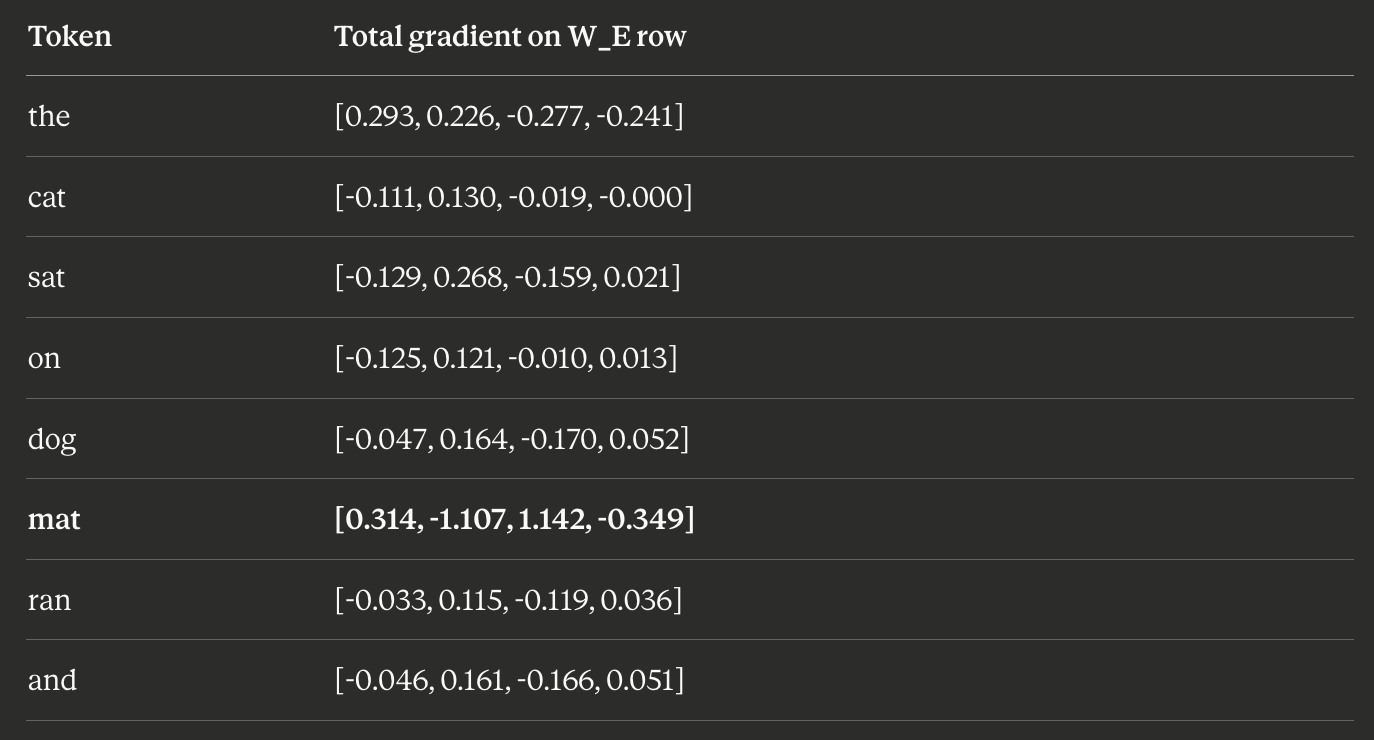
The row for “mat” has by far the largest gradient — because “mat” is the target, and weight tying gave it a massive gradient directly from the output layer. Rows for tokens that didn’t appear in the input (dog, ran, and) only have output-side gradients, from having been considered and partially predicted by the softmax. Rows for tokens that did appear (the, cat, sat, on) have both input-side and output-side contributions.
Step 16: The Weight Update
Applying gradient descent with learning rate η = 0.5 (just like Part 1):
For "mat":
The embedding for “mat” moved substantially. Its second component jumped from 0.4 to 0.954, its third went from 0.2 to -0.371. The direction of the update is aligned with -gradient, which for the output-side contribution is aligned with +h (the final hidden vector from this example). In other words, “mat”’s embedding was pushed toward the current hidden state’s direction. Next time the network sees this context, the dot product between h and “mat”’s embedding will be larger → higher logit → higher probability. The network has learned (a tiny bit) from this example.
For a Q/K/V matrix that got a smaller gradient, the update is tinier. For example, W_V^(2,1):
A microscopic nudge. But applied over billions of training examples, across billions of parameters, these microscopic nudges are exactly what shape a random Transformer into a coherent language model.
The Big Picture
Let’s step back and appreciate what just happened.
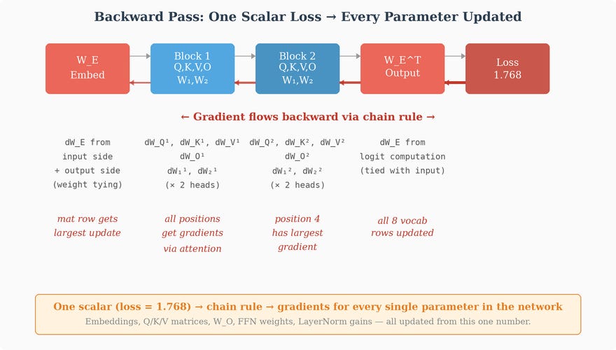
We started with one input sequence, one target token, and a network full of essentially random weights. The model made a weak prediction (17.1% probability on the correct answer). The cross-entropy loss was 1.768. A single scalar — one number.
Backpropagation took that one number and traced it backward through every single parameter in the network:
Every entry of the output head W_E^T (via weight tying, every embedding row)
Every LayerNorm gain and bias (two LNs per block × two blocks + one final = 5 LNs)
Every attention weight matrix: W_Q, W_K, W_V for each of two heads, plus W_O (shared across heads, one per block) — (3 × 2 heads + 1) × 2 blocks = 14 attention matrices
Every FFN weight matrix and bias: W₁, W₂, b_1, b_2 — 4 sets × 2 blocks = 8 FFN parameters
Every entry of the embedding matrix W_E (already counted via weight tying)
Positional encodings (if they were learnable; in our example they were fixed)
Every single one of these parameters got a tiny push, proportional to how much it contributed to the final loss. The push always points in the direction that would, if repeated, reduce the loss — that’s what gradient descent guarantees.
Some observations that should feel powerful by now:
The only signal was -log(0.171) = 1.768. One scalar. Everything else — all 1000+ individual parameter updates — was derived by mechanical application of the chain rule.
“mat”’s embedding got the biggest update. Because of weight tying, the output layer directly pulled “mat”’s row toward the current hidden state vector. Next time this sequence is seen, “mat” will be scored higher at the output.
Every Q/K/V matrix in every head in every block got updated. Not because anyone programmed them to do specific things, but because the chain rule traced the loss back through each of them. If head 7 of block 12 happened to route slightly more attention to the wrong position, its W_Q and W_K will shift slightly to route less that way next time. No one told it which attention pattern is right — the loss implicitly informed it.
The same token at different positions had its gradients accumulated. “The” appeared at positions 0 and 4; both gradient contributions summed into the same row of W_E. This is how the network learns that “the” has some consistent representation across positions — because all its uses push the same row of the embedding matrix.
Weight tying means dual updates for the same matrix. W_E received gradients from both the input side (through the whole network) and the output side (directly from the logit computation). These added together.
Positions 0–3 got non-zero gradients, even though only position 4 produced the loss. This happened via attention: the query at position 4 attended to keys and values at all previous positions, so when the loss propagated back through attention, it flowed to those positions too. This is how “context” tokens get their embeddings shaped — they matter for what came after, so they get a share of the error signal.
Now imagine this entire process, but with:
A vocabulary of 128,000 tokens instead of 8
d_model of 4,096 instead of 4
32 heads per block instead of 2
32 blocks instead of 2
Sequences of thousands of tokens instead of five
Trillions of training examples, processed in batches of thousands at a time
An optimizer like AdamW that tracks running averages of gradients rather than using them directly
A learning rate schedule, gradient clipping, mixed-precision training
The forward and backward passes look the same. The matrices are much bigger. The number of parameter updates per step is in the hundreds of billions. The effect per example is much smaller. But the principle — loss → gradient → update, applied mechanically via the chain rule to every single parameter — is exactly what we just walked through.
That’s how an LLM learns. There’s no secret step. It’s just this, repeated an enormous number of times.
Well and this is it for Part 2. We went from the simple MLP of Part 1 through the entire Transformer architecture — embeddings, attention, feedforward networks, residual connections, normalization — and we traced a complete forward and backward pass through a working (if tiny) model, watching every weight get updated by the chain rule. Next time we will see how a Transformer goes from random weights to a working assistant: pretraining on trillions of tokens, supervised fine-tuning, alignment via RLHF and DPO, and the engineering of inference and serving.
Until next time!